PAGES Magazine articles
Drake McCrimmon![]() 1,2, A. Ihle
1,2, A. Ihle![]() 3, K. Keegan
3, K. Keegan![]() 1 and S. Rupper
1 and S. Rupper![]() 4
4
Firn—old snow slowly densifying into glacial ice—provides valuable information for interpreting ice-core records, modeling meltwater runoff and sea-level rise, and improving our understanding of glacier dynamics through the interpretation of remote-sensing signals.
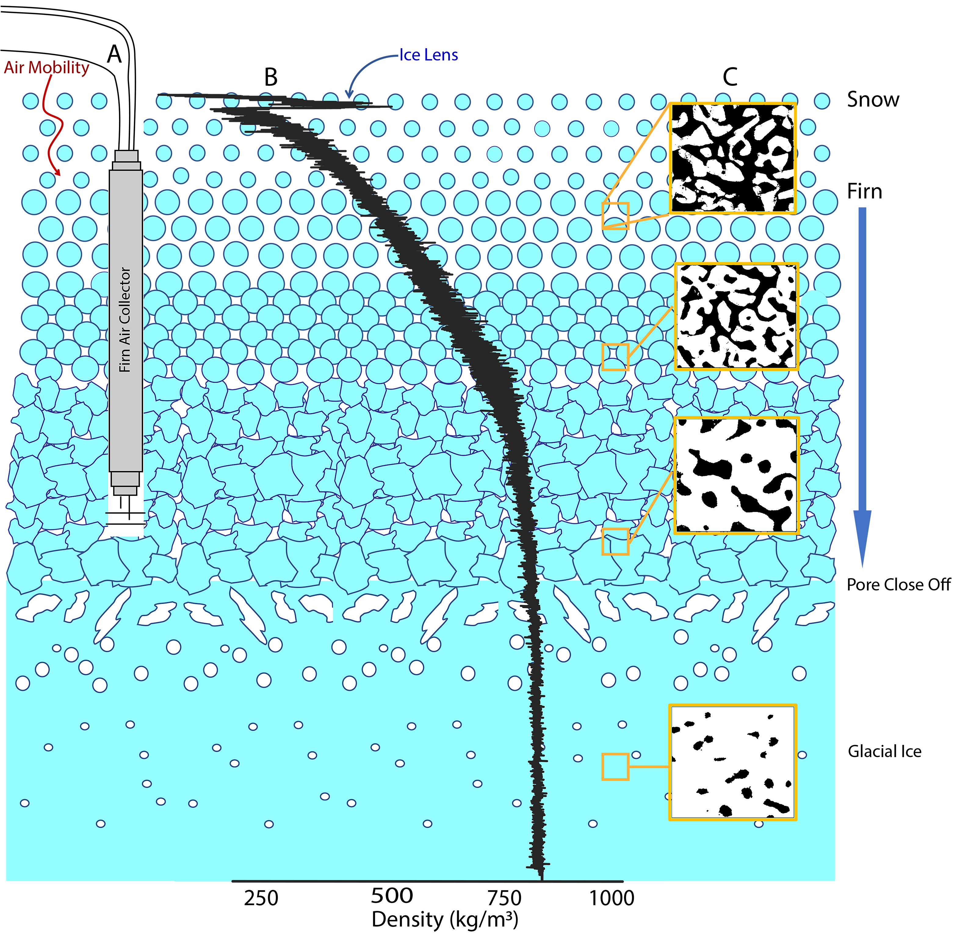
A glacier's cross section can be split into three main components: (1) a low-density layer of fresh snow at the surface, (2) a ~50–100-m-deep transition zone of densifying old snow called firn, and (3) hundreds to thousands of meters of high-density glacial ice at the bottom (Fig. 1). Firn is an important section of a glacier or ice sheet because the densification process and the grain structure impact how climate information is preserved by glacial ice. The microstructure of the firn (the size and shape of snow grains and pore space within the firn, Fig. 1c) influences both the movement and fate of air and water through the firn (Blackford 2007). These processes affect the interpretation of ice-core paleoclimate records, estimation of the capacity for firn to store glacier surface meltwater, and the use of remote sensing to study ice-sheet mass balance.
Interpretation of ice-core records
Gases trapped in ice cores generally reflect the atmosphere at a time in the past, thus allowing scientists to use ice-core gas records to reconstruct past atmospheric composition (Banerjee et al. p. 104), including greenhouse gases, extending back hundreds of thousands of years (Wendt et al. p. 102). The densification of firn is a major control on how gases are preserved in ice, so understanding this process is imperative for studying past climate.
Like surface snow, firn contains pore space between ice grains in which air can flow and liquid water can infiltrate. As firn density increases with burial depth, the space between snow grains shrinks until pores are closed off from one another (Fig. 1b, c). This depth, called the pore close-off depth, is the point when atmospheric gas becomes permanently trapped as bubbles enclosed in ice. Since gas is not trapped until the pore close-off depth, the air that is trapped in bubbles is younger than the surrounding ice (Schwander and Stauffer 1984). This difference in age is called Δage (delta age) and must be known to accurately date gas records from ice cores (Martin et al. p. 100). The Δage makes it possible to determine what the atmospheric composition was at specific points in Earth's climate history. Firn densification models, annual layer counting, and gas-diffusion models allow us to estimate Δage by determining the time it takes for firn to transition into glacial ice, as well as the time it takes for atmospheric gas to move through the firn to reach the pore close-off depth.
 |
|
Figure 1: Background illustration shows the evolution of snow to firn to ice. (A) The firn-air collection apparatus. (B) Example density profile from snow surface through pore close-off to glacial ice (Burgener et al. 2013). (C) Example microCT images at differing densities, with black denoting pore space and white denoting ice grains. |
Since the densification rate of firn is strongly controlled by local climate, empirical firn densification models rely predominantly on site temperature and snow accumulation rate (Herron and Langway 1980). Typically, sites with higher temperatures densify more quickly, and sites with higher accumulation rates tend to have thicker layers of firn. While temperature and accumulation are the strongest controls on the compaction rate and these empirical models predict firn density well, there are other physical processes that also impact firn compaction (Fujita et al. 2014). An active area of firn research is the development of physics-based firn-compaction models that take into account firn microstructure and the underlying physical processes driving firn densification (Keenan et al. 2021). Improved firn-compaction models will allow us to better interpret ice-core paleoclimate records and estimate ice-sheet mass balance from remote sensing, especially in locations where empirical firn compaction models do not predict firn density well enough.
The movement of gas through the firn can also be modeled to help determine Δage. This becomes complicated as atmospheric gas composition is altered as it flows through firn pore spaces. Several physical processes alter how gas moves through firn, such as the settling of heavy gasses due to gravity and temperature-gradient-driven gas separation (Severinghaus et al. 1998). This means that the heavier isotopes of gases settle deeper into the firn and also towards cooler temperatures. This results in a slight difference in gas composition between when the gas enters the firn column and when the gas reaches pore close-off. Gas diffusion models are tuned to many different gas species in order to accurately model the movement of different gasses through firn (Buizert et al. 2012). Optimizing these models allows researchers to correct for the change in gas composition within the firn and improve the age estimation of gases. In addition, the air that is traveling through the firn column can also be collected and measured to understand the atmospheric composition in recent history (Fig. 1a; Butler et al. 1999). This firn air is a link between current atmospheric composition and that which is trapped within ice-core bubbles, which may be hundreds to thousands of years old.
Modeling meltwater runoff and sea-level rise
 |
|
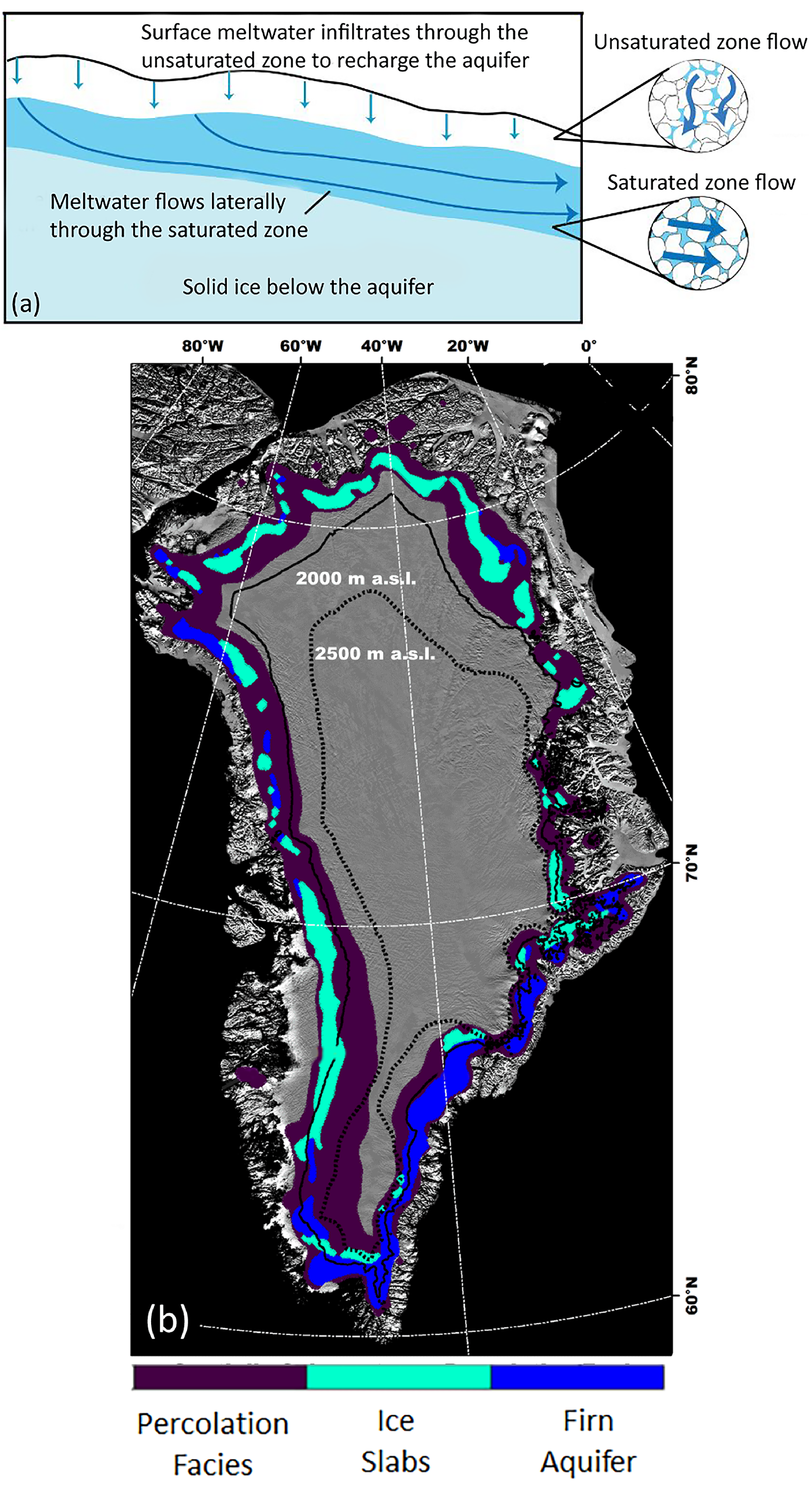
Figure 2: (A) A conceptual illustration of meltwater percolation into a firn aquifer (adapted from Miller et al. in review); and (B) Current firn aquifer extent in Greenland (adapted from Miller et al. 2022). |
The fate of ice-sheet surface meltwater depends strongly on firn. Instead of running off the ice sheet directly into the ocean, surface meltwater can percolate into the open pore spaces in firn, leading to the development of firn aquifers (Fig. 2a). Remote sensing has shown that there are large areas on both the Greenland and Antarctic ice sheets that have conditions conducive to forming firn aquifers. These conditions include high rates of melting and snow accumulation (Forster et al. 2014). High snow accumulation leads to a thicker layer of firn pore space and insulation to retain meltwater (Kuipers Munneke et al. 2014). In Greenland, large firn aquifers are found on the perimeter of the ice sheet (Fig. 2b) where such conditions are met (Koenig et al. 2014; Miller et al. 2022). Because firn aquifers can slow or entirely prevent meltwater runoff, determining the conditions under which firn aquifers develop will ultimately lead to more accurate estimates of how much surface meltwater will be stored within the firn, versus how much will runoff to the sea (Christ et al. p. 116).
Remote sensing for ice-sheet mass balance
Changes in the thickness and density of firn are a significant uncertainty in estimates of ice-sheet mass change using satellite measurements of surface elevation (Smith et al. 2020). For satellite measurements using microwave radiation, scattering related to snow grain and pore sizes can limit the ability of microwave radiation to penetrate into the ice sheet (Rott et al. 1993). This scattering complicates the use of remote sensing to understand the underlying structure of firn, its meltwater buffering capacity, and changes in ice-sheet surface elevation. Current work aims to use firn microstructure to inform the interpretation of microwave remote sensing on ice sheets in order to improve our understanding of ice-sheet mass balance, both today and in a warming future (Keenan et al. 2021).
Conclusion
Understanding the firn transitional zone is crucial to the accurate reconstruction of past climates, realizing the fate of ice-sheet surface meltwater, and improving estimates of ice-sheet mass balance. Firn provides an important link between processes in the modern atmosphere and ancient atmosphere that is trapped in deep glacial ice. The structure of firn also has major controls on the interpretation of remote sensing signals of glacier surfaces. Ultimately, improving our understanding of firn will deepen our insight of many processes on glaciers and ice sheets.
affiliationS
1Department of Geological Sciences and Engineering, University of Nevada Reno, USA
2Division of Hydrologic Sciences, Desert Research Institute, Reno, NV, USA
3Department of Earth and Environmental Sciences, University of Rochester, NY, USA
4Department of Geography, University of Utah, Salt Lake City, USA
contact
Drake McCrimmon: drake.mccrimmon@dri.edu
references
Blackford JR (2007) J Phys D Appl Phys 40: R355-R385
Buizert C et al. (2012) Atmos Chem Phys 12: 4259-4277
Burgener L et al. (2013) J Geophys Res Atmos 118: 4205-4216
Butler JH et al. (1999) Nature 399: 749-755
Forster RR et al. (2014) Nat Geosci 7: 95-98
Fujita S et al. (2014) J Glaciol 60: 905-921
Herron MM, Langway CC Jr (1980) J Glaciol 25: 373-385
Keenan E et al. (2021) Cryosphere 15: 1065-1085
Koenig LS et al. (2014) Geophys Res Lett 41: 81-85
Kuipers Munneke P et al. (2014) Geophys Res Lett 41: 476-483
Miller JZ et al. (2022) Cryosphere 16: 103-125
Rott H et al. (1993) Ann Glaciol 17: 337-343
Schwander J, Stauffer B (1984) Nature 311: 45-47
Madelyne C. Willis1,2, N. Chellman3 and H.J. Smith2,4
This article highlights the state of knowledge of glacial microorganisms, focusing on englacial habitats, challenges associated with studying cells in these environments, and considerations for future ice-core projects seeking to advance biological studies as part of their scientific objectives.
Once thought to be inhospitable to life, glaciers and ice sheets are now considered microbially dominated biomes. Anesio et al. (2017) estimated there may be on the order of 1029 cells in all of Earth's glaciers and ice sheets, on the same order of magnitude as the reported total cell abundance for all aquatic systems on Earth (1.2 x 1029 cells; Whitman et al. 1998). Originally assumed to be preserved in a dormant state, studies over the past 20 years have demonstrated many of these cells are likely viable, and their presence and function have profound implications for a wide range of scientific fields including paleoclimatology, bioprospecting, and exobiology (D'Andrilli et al. 2017; Balcazar et al. 2015; Tung et al. 2005). Despite this shift to a perception of glaciers as habitable, methodological challenges and the fact that biological studies are often secondary to other scientific goals on deep ice coring projects have limited the study of microorganisms in englacial ice. Looking forward, recent advancements in lab- and field-based methods have created new opportunities for investigating life in these unique ecosystems.
Implications of ice as a habitable space
Glaciers and ice sheets contain liquid water features which may be habitable for microorganisms throughout all three glacial zones (supraglacial, englacial and subglacial) (Boetius et al. 2015). Investigations of glacier microbial communities have focused primarily on the relatively dynamic supraglacial and subglacial zones, emphasizing surface features such as ephemeral meltwater streams and ponds, and cryoconites (depressions in the surface filled with dust and liquid water; Cook et al. 2015), and subglacial hydrological systems (Mikucki et al. 2016; Walcott et al. p. 114). Much less is known about the biology of englacial ecosystems, despite these environments comprising the bulk of glacier ice mass (Boetius et al. 2015).
Within the englacial environment, habitable spaces may be found on the micron scale in water-filled pore spaces between ice crystals and in thin layers of liquid water surrounding dust particles trapped within ice (Tung et al. 2005). While a lack of energy sources and nutrients in these microhabitats may inhibit optimal growth, it is widely accepted that under these conditions microbes can maintain the low levels of activity needed to support basic housekeeping functions (Dieser et al. 2013). These functions, for example DNA repair, allow the cell to remain viable and may result in the uptake or production of some greenhouse gases (Fig. 1). Over geologic timescales, the activity required for cellular maintenance may be adequate to offset ice-core gas records by producing anomalous, non-atmospheric signals of gases e.g. nitrous oxide, methane, and carbon monoxide (Miteva et al. 2016; Fain et al. 2022; Banerjee et al. p. 104). At present, our understanding of in-situ microbial activity within glacier ice is limited to either theoretical (Tung et al. 2005), or in-vitro laboratory studies (Dieser et al. 2013); there has been no direct measure of microbial activity within deep glacial ice. Studies providing empirical evidence of microbial activity or quiescence would facilitate more robust paleoclimatic reconstructions, and understanding the resilience of these organisms may inform our search for life on Mars or other planetary environments containing water ice.
 |
|
Figure 1: Schematic of ice-core gas records and corresponding in-situ microbial metabolic strategies illustrating the potential for microbial metabolic activity to impact paleoclimatic records. Methanogenesis results in the release of methane (CH4) outside of the cell and chemolithoautotrophy results in the consumption of carbon dioxide (CO2). |
Challenges and considerations
The gap in knowledge regarding in-situ biological activity is largely due to the difficulty of performing biological measurements on ice-core samples. The primary hurdle for most studies is the inherently low biomass within glacier ice. Although cell concentrations as high as 106 cells/mL have been reported (Miteva et al. 2016), these high numbers correlate with high dust concentrations and, in general, englacial cell numbers tend to be much lower: between 101 and 104 cells/mL (Santibáñez et al. 2018).
The challenge of low biomass is exacerbated by limited sample volumes available from deep ice-core projects, contamination, and insufficient sensitivity of analytical methods. Core fracturing is a source of contamination that can easily be introduced during ice-core breaking and inconsistent temperature storage. Contamination from mechanical drilling practices that use hydrocarbon-based drilling fluids is of particular concern, as these fluids can contaminate both cores and the subglacial environment. Existing ice-core decontamination protocols are effective but can result in appreciable sample loss. Once samples have been transported to the laboratory and decontaminated, many traditional microbiological approaches lack the sensitivity required for low biomass englacial ice. Depending on final cell concentrations, relatively large sample volumes (5–500 mL meltwater) are often required for these approaches.
Recent developments
Fortunately, recent advancements in drilling systems, microbial analytical methods, and in-situ technology make this an exciting moment for probing questions about microbiology in ice. Hot-water drilling and air-reverse circulation are alternatives to mechanical drilling with organic fluids and have been demonstrated to be effective and to limit contamination (Talalay and Hong 2021). In addition, engineering solutions which prevent vertical and diagonal fracturing of cores during drilling processes preserve more core sections suitable for microbial analysis (Talalay and Hong 2021). Use of a replicate ice-coring system can provide additional sample volume at depths with high community demand for core sections by drilling replicate cores slightly deviated from the original borehole. Use of these systems could provide the sample volume required for microbial analyses.
In the lab, continuous flow analysis provides detailed temporal resolution of decontaminated ice (Santibáñez et al. 2018), which is particularly useful for biological applications to monitor contamination (e.g. the detection of drilling fluids or other anomalies). Innovative and highly sensitive analytical techniques, such as nanoSIMS, stable isotope probing, and other next-generation physiology measurements can reveal cellular function on the single-cell level (Fig. 2). Excitingly for ice-core studies, many of these next-generation approaches are also nondestructive, which enables crucial downstream analyses of individual cells such as cultivation, sequencing, and "omics" approaches. These methods have been demonstrated for studies of microbial diversity and physiology in a variety of low-biomass natural samples; however, they have yet to be applied to studies of deep ice cores. Hatzenpichler et al. (2020) provide a full review of next-generation physiology techniques.
 |
|
Figure 2: Schematic of ice-core gas records and corresponding in-situ microbial metabolic strategies illustrating the potential for microbial metabolic activity to impact paleoclimatic records. Methanogenesis results in the release of methane (CH4) outside of the cell and chemolithoautotrophy results in the consumption of carbon dioxide (CO2). |
Field-deployable technologies are complementary to lab-based methods and are capable of detecting cells or biorelevant compounds within the solid ice matrix (Eshelman et al. 2019). Cells and compounds that may become too dilute once melted (ex: 102–104 cells/mL), can be concentrated at detectable levels (106–108 cells/mL) within the grain boundaries of solid ice (Mader et al. 2006). Since most biological measurements traditionally require samples to be melted before analysis, the development of non-destructive technologies could result in new approaches to studying englaciated life in situ. Additionally, the incorporation of these technologies into the drilling process creates the potential for real-time data collection within the ice borehole. This could provide a means to detect areas of interest based on organic or microbial content during the drilling process and allow for data-driven decision-making during ice-core collection, for instance in determining the depths of interest for replicate coring.
Conclusion
Ice-core research has traditionally focused on reconstructing Earth's climate and environmental history using measurements of stable water isotopes, gases, and other inorganic compounds preserved within the ice. However, we now have the capability to better understand the abundance and function of microbial communities in ice. These organisms may have a profound impact on paleoclimatic records preserved in ice chemistry, may be used as additional indicators of past depositional events related to climate, and may serve as proxies for life in extraterrestrial water ice elsewhere in our solar system. If considerations for biological measurements are taken into account early in planning future drilling projects, there will be greater opportunities to discover the englacial microbiome.
Acknowledgements
The authors would like to thank Foreman Lab Group members for discussions about life in ice and comments that improved the manuscript. M. Willis, and H. Smith are supported by NSF Antarctic Research (2037963).
affiliationS
1Department of Land Resources and Environmental Science, Montana State University, Bozeman, USA
2Center for Biofilm Engineering, Montana State University, Bozeman, USA
3Division of Hydrologic Sciences, Desert Research Institute, Reno, NV, USA
4Department of Microbiology and Cell Biology, Montana State University, Bozeman, USA
contact
Madelyne Willis: madie.willis@gmail.com
references
Anesio AM et al. (2017) NPJ Biofilms Microbiomes 3: 10
Balcazar W et al. (2015) Microbiol Res 177: 1-7
Boetius A et al. (2015) Nat Rev Microbiol 11: 677-690
Cook J et al. (2015) Prog Phys Geogr 40: 66-111
D'Andrilli J et al. (2017) Geochem Perspec Lett 4: 29-34
Dieser M et al. (2013) Appl Environ Microbiol 24: 7662-7668
Eshelman EJ et al. (2019) Astrobiology 19: 771-784
Faïn X et al. (2022) Clim Past 18: 631-647
Hatzenpichler R et al. (2020) Nat Rev Microbiol 18: 241-256
Mader HM et al. (2006) Geology 34: 169-172
Mikucki JA et al. (2016) Philos Trans R Soc A 374: 20140290
Miteva V et al. (2016) Geomicrobiol J 33: 647-660
Santibáñez PA et al. (2018) Glob Chang Biol 24: 2182-2197
Talalay PG, Hong J (2021) Ann Glaciol 62: 143-156
Tung HC et al. (2005) Proc Natl Acad Sci USA 102: 18,292-18,296
Whitman WB et al. (1998) Proc Natl Acad Sci USA 95: 6578–6583
Sophia M. Wensman![]() 1, J.D. Morgan2 and K. Keegan
1, J.D. Morgan2 and K. Keegan![]() 3
3
Ice cores can provide high-resolution records of anthropogenic activities, observable in gas and impurity records, for at least the last few millennia. Such archives demonstrate the ubiquity of human influence and the importance of legislation in mitigating these impacts.
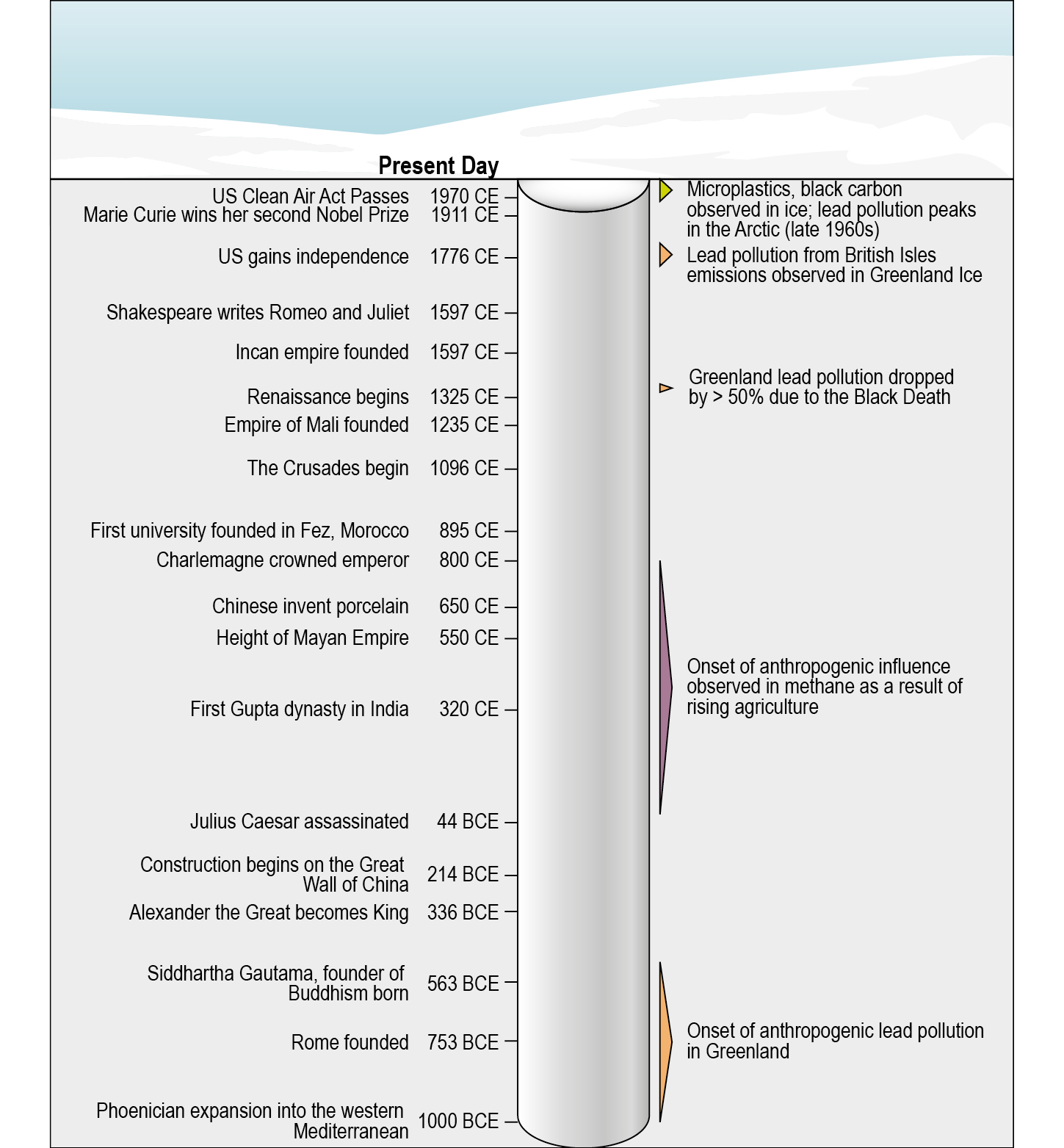
Ice cores archive direct and proxy records of human impacts on the environment. The impact of human activity on the environment is clearly visible in ice cores as: increasing concentrations of methane and other greenhouse gases (e.g. Banerjee et al. p. 104; Mitchell et al. 2013); spikes in radionuclides from atomic bomb explosions (e.g. Gabrielli and Vallelonga 2015); and elevated concentrations of pollutants like lead, microplastics, and black carbon (e.g. Materić et al. 2022; Gabrielli and Vallelonga 2015; Fig. 1).
Ice-core records also extend much further into the past than modern observations, revealing the widespread extent of historical anthropogenic impacts. Here, we focus on methane and lead, two chemical species that record some of the earliest ice-core evidence of human impacts on the environment, beginning at least 2500 years ago. Additionally, we discuss examples of ice-core records that show the impact of remediation actions including legislation and technological advancements in reducing anthropogenic influence.
Methane emissions from early agriculture
Ice cores record changes in the composition of the atmosphere in air bubbles that get trapped as snow and ice accumulate. Air bubbles in ice cores from both Greenland and Antarctica record a steady 100-ppb increase in atmospheric methane concentrations beginning around 5000 years ago. There has been much debate about whether this reflects natural variability or is evidence of early human influence on the environment via land clearance and agriculture, such as rice and livestock farming. Fortunately, ice cores offer tools to investigate this question. For example, the difference in methane concentration between Arctic and Antarctic ice cores tells us which hemisphere has larger emissions. Additionally, the isotopic composition of methane in the ice preserves a fingerprint of where and how it was produced. Using these techniques, ice cores reveal that the increase between 5000 and 2000 years ago likely came from stronger monsoons in the Southern Hemisphere, rather than rice farming in East Asia (Beck et al. 2018). Studying these natural variations allows us to better identify the impact of human activity.
Anthropogenic methane emissions became truly significant during the last 2000 years (Fig. 1). During this period, the rise in methane concentrations in the ice cores cannot be explained without the increase of emissions from human activity, such as rice and cattle farming and decomposition in landfills (Mitchell et al. 2013). The sensitivity of methane emissions to human population and industry is also evident in the sharp dips in Northern Hemisphere emissions coinciding with the fall of the Roman Empire and Han Dynasty (Sapart et al. 2012), the arrival of the Black Plague in Asia (Mitchell et al. 2013), and the deaths of Indigenous Americans resulting from European invasion and subsequent disease introduction (Ferretti et al. 2005).
Human impacts on lead pollution
 |
|
Figure 1: Ice-core records of environmental pollutants before and after enactment of the US Clean Air Act in 1970 (dashed line). (A) Lead flux from southern Greenland ice cores (McConnell et al. 2019); (B) Summit, Greenland, sulfate concentrations (Geng et al. 2014); (C) Acidity levels from northern Greenland (Maselli et al. 2017); and (D) Mercury concentrations from Upper Fremont Glacier in Wyoming, USA (Chellman et al. 2017). |
Anthropogenic emissions of lead, a toxic heavy metal emitted from industrial activities including mining and fossil-fuel burning, are first observed in Arctic ice cores approximately 3000 years ago (e.g. Murozumi et al. 1969), with earliest evidence of lead pollution attributed to the expansion of the Phoenician society (McConnell et al. 2018). Antarctic ice cores record anthropogenic lead pollution only during the last 130 years due to lower emissions in the Southern Hemisphere, with earliest emissions from mining and smelting of lead ores in Australia (Vallelonga et al. 2002). High-resolution ice-core records demonstrate the sensitivity of ice cores to year-to-year and decade-to-decade changes in anthropogenic emissions corresponding to major historical events including plagues, wars, and periods of economic stability (e.g. McConnell et al. 2018).
Arctic lead pollution rose rapidly during the industrial period, peaking in the 1960s, when leaded gasoline use was most prevalent. Indeed, Greenland ice cores indicate that Arctic lead pollution increased 250- to 300-fold between the Early Middle Ages and the 1960s (McConnell et al. 2019), with lead isotopic records suggesting predominantly US-derived sources (e.g. Wensman et al. 2022). Clair Patterson and colleagues first noted large-scale increases in lead pollution in Greenland ice associated with leaded gasoline use (e.g. Murozumi et al. 1969). Using ice cores to determine pre-industrial levels of lead pollution, they demonstrated that increased lead deposition was caused by anthropogenic emissions; these results influenced the passage of the US Clean Air Act in 1970.
Impact of environmental legislation
Following enactment of legislation in North America and Europe in the 1970s and 80s, ice cores show lead pollution declined rapidly, with current levels approximately 80% lower than during the height of leaded gasoline use, though deposition remains 60-fold higher than pre-industrial levels (McConnell et al. 2019; Fig. 2a). In addition to decreases in lead pollution, other pollutants also record evidence of positive human impacts following the US Clean Air Act, and similar legislation enacted around the world (e.g. Environment Action Programme in Europe). One example is the concentration of sulfates in ice from Summit Station in central Greenland. Sulfates primarily originate from coal burning, and therefore their atmospheric concentration increased after the Industrial Revolution. This increase was recorded in the Greenland Ice Sheet (Geng et al. 2014) until the enactment of the Clean Air Act, following which ice-core sulfate concentrations returned to pre-industrial levels (Fig. 2b). Measurements in ice cores also show decreased acidity levels following the Clean Air Act and ensuing market-based cap-and-trade systems (which set limits on allowable pollutant emissions for companies) for sulfur dioxide and nitrogen oxides, which are key chemical species in the formation of acid rain, produced as a byproduct of fossil-fuel burning (Fig. 2c; Maselli et al. 2017; Geng et al. 2014). At Upper Fremont Glacier in Wyoming, USA, there has been a sharp decrease in mercury levels (a toxic heavy metal and anthropogenic pollutant) recorded in the ice since the 1970s, due to the lack of recent volcanic activity and legislation requiring the addition of pollutant scrubbers to industrial flue-gas stacks (Fig. 2d; Chellman et al. 2017).
 |
|
Figure 2: Ice-core records of environmental pollutants before and after enactment of the US Clean Air Act in 1970 (dashed line). (A) Lead flux from southern Greenland ice cores (McConnell et al. 2019); (B) Summit, Greenland, sulfate concentrations (Geng et al. 2014); (C) Acidity levels from northern Greenland (Maselli et al. 2017); and (D) Mercury concentrations from Upper Fremont Glacier in Wyoming, USA (Chellman et al. 2017). |
Ice-core records of pollutants demonstrate the importance of legislation regulating anthropogenic emissions and suggest further environmental legislation may result in continued reductions in anthropogenic emissions. As far as we are aware, no ice-core studies to date have incorporated Indigenous knowledge in interpretation of ice-core data; however, Indigenous experts can enhance our understanding of the role humans have played in shaping the environment and improve effectiveness of legislation. Previous examples of studies within the Earth sciences provide mechanisms for working across knowledge systems to create respectful, inclusive, and effective collaborations with Indigenous experts (e.g. Hill et al. 2020), including tracking sea-ice extent and thickness (Tremblay et al. 2008). Such collaborations could be impactful in ice-core science in, for example, expanding understanding of early pollution histories or impacts of long-range pollution transport, as observed in ice cores, on Indigenous Arctic populations.
Conclusion
The exponential acceleration and vast extent of anthropogenic disruption of the environment is uniquely recorded by a vast array of ice-core datasets. The historical context ice cores provide, by extending contemporary measurements into the past, will continue to be invaluable as previously undiscovered impacts emerge. Ice cores provide unique long-term records, highlighting both the level to which humans have altered remote environments, and the role legislation can have in reducing human influence.
affiliationS
1Division of Hydrologic Sciences, Desert Research Institute, Reno, NV, USA
2Scripps Institution of Oceanography, University of California San Diego, La Jolla, USA
3University of Nevada Reno, USA
contact
Sophia Wensman: sophia.wensman@dri.edu
references
Beck J et al. (2018) Biogeosciences 15: 7155-7175
Chellman N et al. (2017) Environ Sci Technol 51: 4230-4238
Ferretti DF et al. (2005) Science 309: 1714-1717
Geng L et al. (2014) Proc Natl Acad Sci USA 111: 5808-5812
Hill R et al. (2020) Curr Opin Environ Sust 43: 8-20
Maselli OJ et al. (2017) Clim Past 13: 39-59
Materić D et al. (2022) Environ Res 208: 112741
McConnell JR et al. (2018) Proc Natl Acad Sci USA 115: 5726-5731
McConnell JR et al. (2019) Proc Natl Acad Sci USA 116: 14,910-14,915
Mitchell L et al. (2013) Science 342: 964-966
Murozumi M et al. (1969) Geochim Cosmochim Acta 33: 1247-1294
Sapart CJ et al. (2012) Nature 490: 85-88
Tremblay M et al. (2008) Arctic 61: 27-34
Vallelonga P et al. (2002) Earth Planet Sci Lett 204: 291-306
Fire trapped in ice: An introduction to biomass burning records from high-alpine and polar ice cores
Sandra O. Brugger![]() 1, Liam Kirkpatrick
1, Liam Kirkpatrick![]() 2 and Laurence Y. Yeung
2 and Laurence Y. Yeung![]() 3
3
All authors contributed equally and are considered joint first authors.
Paleofire research is crucial for understanding long-term wildfire trends for fire and air quality management. Future work should close geographic gaps and incorporate cross-disciplinary collaborations for a holistic understanding of wildfires and their role in the climate system.
Fires are a unique element of the climate system. They are highly sensitive to regional climate, vegetation, and human factors, and serve as a significant driver of global climate and atmospheric composition (Legrand et al. 2016). Recent years were marked by devastating fire seasons worldwide with severe consequences for human health, economies, and ecosystems across continents. Yet, current biomass burning trends are a result of complex interactions between changing land-use practices, ecosystem dynamics, and climatic factors. Paleorecords provide a crucial context for both trends and drivers of burning, which help us understand how fires are changing now and how they might change in the future.
Efforts to build paleofire records began almost 100 years ago with charcoal analyses from Greenland sediments (Stutzer 1929). Early efforts to study paleofire in ice cores focused on black carbon (soot), but modern ice-core paleofire studies employ a range of proxies for biomass burning (Legrand et al. 2016) and utilize the long, accurate chronologies unique to ice cores (Martin et al. p. 100).
Paleofire proxies in ice cores
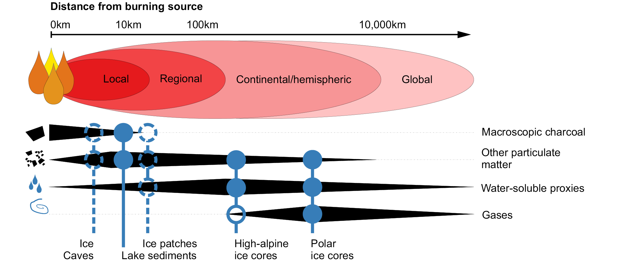
Fires yield products that are transported from the fire source region and deposited on ice. These fire tracers are preserved in the ice matrix as particulate matter, water-soluble species, and gases. They have varying levels of dilution, preservation potential, and specificity to biomass burning (Fig. 1). For example, black carbon is comprised of submicron-sized particles which can be produced by incomplete biomass combustion or by fossil-fuel burning (McConnell et al. 2007). Ammonium and potassium ions (which are water-soluble) also have multiple sources and thus correlate with wildfire activity only after accounting for the naturally occurring background (Rubino et al. 2016). Certain soluble organic molecules can present greater specificity to biomass burning—levoglucosan, for example (Simoneit 2002)—but atmospheric processes in gaseous and aqueous phases (Li et al. 2021) limit how well one can quantify past fire emissions from these ice-core records at present. Other small organic molecules produced in fires, such as acetylene and ethane (gaseous proxies), have simpler and better-understood atmospheric budgets that result in additional insights into burning history (Nicewonger et al. 2020). Finally, the isotopic compositions of gases such as methane are sensitive to changes in their emission sources, facilitating unique constraints on hemispheric- and global-scale biomass burning (Bock et al. 2017).
Note that while each proxy system has its unique advantages and shortcomings, the evidence for changes in paleofire regimes has been corroborated by multiple proxies in many cases, lending confidence to qualitative trends inferred for the last 2000 years. Recent reviews by Legrand et al. (2016) and Rubino et al. (2016) provide more comprehensive discussions about individual proxy systems.
 |
|
Figure 1: Atmospheric footprint of fire tracers in natural archives. Full circles indicate established fire proxies in a certain archive. Dashed circles indicate future directions of proxies in a certain archive. Note that high-fidelity gas records in high-alpine glaciers have been elusive. |
Spatial coverage of ice-core paleofire records
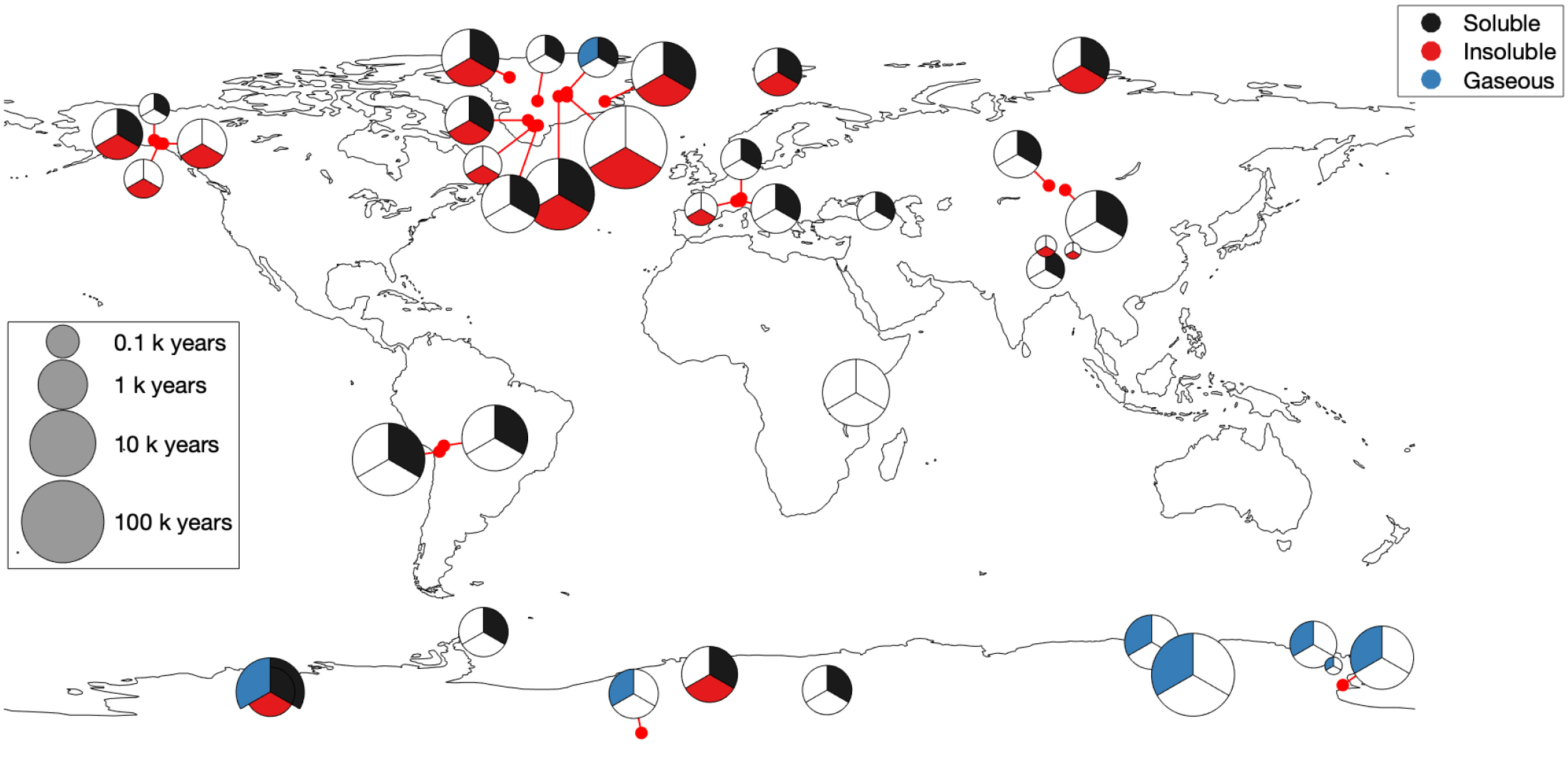
The spatial distribution of available ice cores is skewed towards the poles, with a few high-alpine ice cores in temperate and tropical mountain ranges (Davidge et al. p. 98). Likewise, the coverage of ice-core-based paleofire reconstructions in polar regions is relatively extensive and includes many different particulate, water-soluble, and gaseous proxies (Fig. 2). Outside the polar regions, several multi- proxy paleofire reconstructions have been developed from the tropical South American Andes and the Himalayan region showing millennial-scale changes in fire regimes. Large-scale fire reconstructions based on black carbon, ammonium, nitrate, and microscopic charcoal in the temperate regions are concentrated in the Altai mountains in Central Asia and the European Alps. However, some regions with massive modern fire activity have not yet been investigated. For example, to our knowledge, there is not a single study investigating fire activity trends from the African continent, although Kilimanjaro, Tanzania, could provide a suitable ice archive.
Insights from ice fire records
Ice-core paleofire records show important trends for the last 2000 years, although a few records provide context from the late Pleistocene glacial cycles (Fig. 2). Two broad trends from these records are notable. First, decadal- to millennial-scale variability in fire activity has been inferred for the past 2000 years, arising from human activities and climatic driving forces. For example, global fire activity was higher during the Medieval Climate Anomaly (ca. 950–1250 CE) and then decreased into the Little Ice Age (ca. 1400–1850 CE, Rubino et al. 2016). Second, on glacial–interglacial timescales, large variations in land ice coverage, hydroclimate, and vegetation yielded higher amplitude changes in biomass burning compared to the Holocene (ca. 9700 BCE–modern). The stable isotopic composition of methane suggests that global biomass burning emissions increased between 115 kyr BP and 18 kyr BP, perhaps due to the extinction of megaherbivores that led to an increase in plant biomass (Bock et al. 2017). However, much remains to be learned about glacial–interglacial trends in biomass burning.
Future directions and conclusions
Ice-core records have most clearly illuminated the history of Northern Hemisphere paleofires over the past ~2000 years. Yet, key records from the Southern Hemisphere and Africa are still missing. In addition, proxy measures distinguishing between paleofire frequency and severity, on local to global scales, are needed. Filling in these gaps will improve our understanding of the relationship between fire, climate, ecosystems, and human activities. Fortunately, ice-core science is well suited for cross-disciplinary syntheses, which integrate paleofire reconstructions with atmospheric and ecological dynamics and past human impacts. Such research may incorporate multidisciplinary approaches and collaborations with experts in other fields.
 |
|
Figure 2: The distribution, temporal range, and type of paleofire records derived from ice cores. White sections indicate sites with a missing group of proxies. Note Kilimanjaro, shown as a notable missing archive for paleofire reconstructions. References to original datasets available from Brugger et al. (2022). |
New ice-core archives, such as from ice caves or alpine ice patches (Leunda et al. 2019), that have already yielded promising ice-core records could extend the spatial coverage of ice-core-based biomass-burning reconstructions. Comparison of paleofire records from ice cores with peat-, lake- and marine-sediment cores, as well as tree rings, also helps close geographic gaps and adds to a holistic understanding of past fire regimes. Sharing methodologies such as the application of black carbon methods to lake sediments (Chellman et al. 2018) and incorporating the measurements of traditional sediment–charcoal methods in ice-core science may facilitate comparison across paleoarchives. Due to the much larger particle size, charcoal fragments have a much shorter atmospheric lifetime and, thus, provide more local information compared to the more regional records derived from the smaller particles and gases recorded in ice cores (Fig. 1).
The use of multiple approaches is key to understanding regional patterns of past fire dynamics, fire severity, and sources for the individual biomass-burning proxies. Disentangling proxy sources is particularly important in the industrial period, given the influence of fossil-fuel and land-use emissions on individual fire proxies. Indeed, humanity's relationship with fire has likely been as variable as the cultures that comprise it; through time and space, social needs, traditions, and technological advances together have shaped the role of fire in society. Indigenous and local communities, in particular, should be included in the current fire dialogue to understand the role of fire in cultural traditions and oral histories. The broader paleofire community in the Global Paleofire Working Group highlighted the importance of combining paleofire research with traditional and Indigenous knowledge systems (Colombaroli et al. 2018).
We conclude that research on establishing paleofire records from ice cores is a relatively young field that is rapidly evolving. It has the potential to provide a much-needed long-term global and regional context for current fire adaptation strategies of society and natural systems (Watts and Brugger 2022) in a rapidly changing climate.
affiliationS
1Division of Hydrologic Sciences, Desert Research Institute, Reno, NV, USA
2Department of Earth Science, Dartmouth College, Hanover, NH, USA
3Departments of Earth, Environmental and Planetary Sciences and Chemistry, Rice University, Houston, TX, USA
contact
Sandra O. Brugger: sandra.brugger@dri.edu
references
Bock M et al. (2017) Proc Natl Acad Sci USA 114: E5778-E5786
Brugger SO et al. (2022) Zenodo, doi:10.5281/zenodo.6850553
Chellman NJ et al. (2018) Limnol Oceanogr 16: 711-721
Colombaroli D et al. (2018) PAGES Mag 26: 89
Legrand M et al. (2016) Clim Past 12: 2033-2059
Leunda M et al. (2019) J Ecol 107: 814-828
Li Y et al. (2021) Environ Sci Technol 55: 5525-5536
McConnell JR et al. (2007) Science 317: 1381-1384
Nicewonger MR et al. (2020) J Geophys Res Atmos 125: e2020JD032932
Rubino M et al. (2016) Anthr Rev 3: 140-162
Simoneit BRT (2002) Appl Geochem 17: 129-162
Stutzer O (Ed) (1929) Fusit–Vorkommen, Entstehung und praktische Bedeutung der Faserkohle. Verlag von Ferdinand Enke, 139 pp
Asmita Banerjee![]() 1, Ben E. Riddell-Young
1, Ben E. Riddell-Young![]() 2 and Ursula A. Jongebloed
2 and Ursula A. Jongebloed![]() 3
3
All authors contributed equally and are considered joint first authors.
Ice cores record fundamental information about past atmospheric composition and chemistry, its intricate relationship with global climate, and recent changes to the atmosphere's composition due to anthropogenic activities.
As snow accumulates and compacts on ice sheets, ambient air is trapped within the ice, making glacial ice a direct archive of past atmospheric composition (McCrimmon et al. p. 112). The extraction and measurement of gases trapped in ice cores provide continuous, direct observations of atmospheric composition going back hundreds of thousands of years. These records show changes in atmospheric composition on timescales ranging from decades to hundreds of millennia (Martin et al. p. 100). Ice cores have provided high-resolution records of greenhouse gas (GHG) concentrations including carbon dioxide (CO2) and methane (CH4), and their influence on, and relation to, global climate.
In addition to trapped gases, ice cores also provide a unique archive of major ions and non-gaseous compounds including sulfate (SO42-, nitrate (NO3-), and halogens (e.g. chloride, bromide, iodide); atmospheric acidity; and other measurements that provide information about atmospheric chemistry and anthropogenic pollution. In the following sections, we describe these ice-core records of Earth's atmosphere.
Long-term records of greenhouse gases
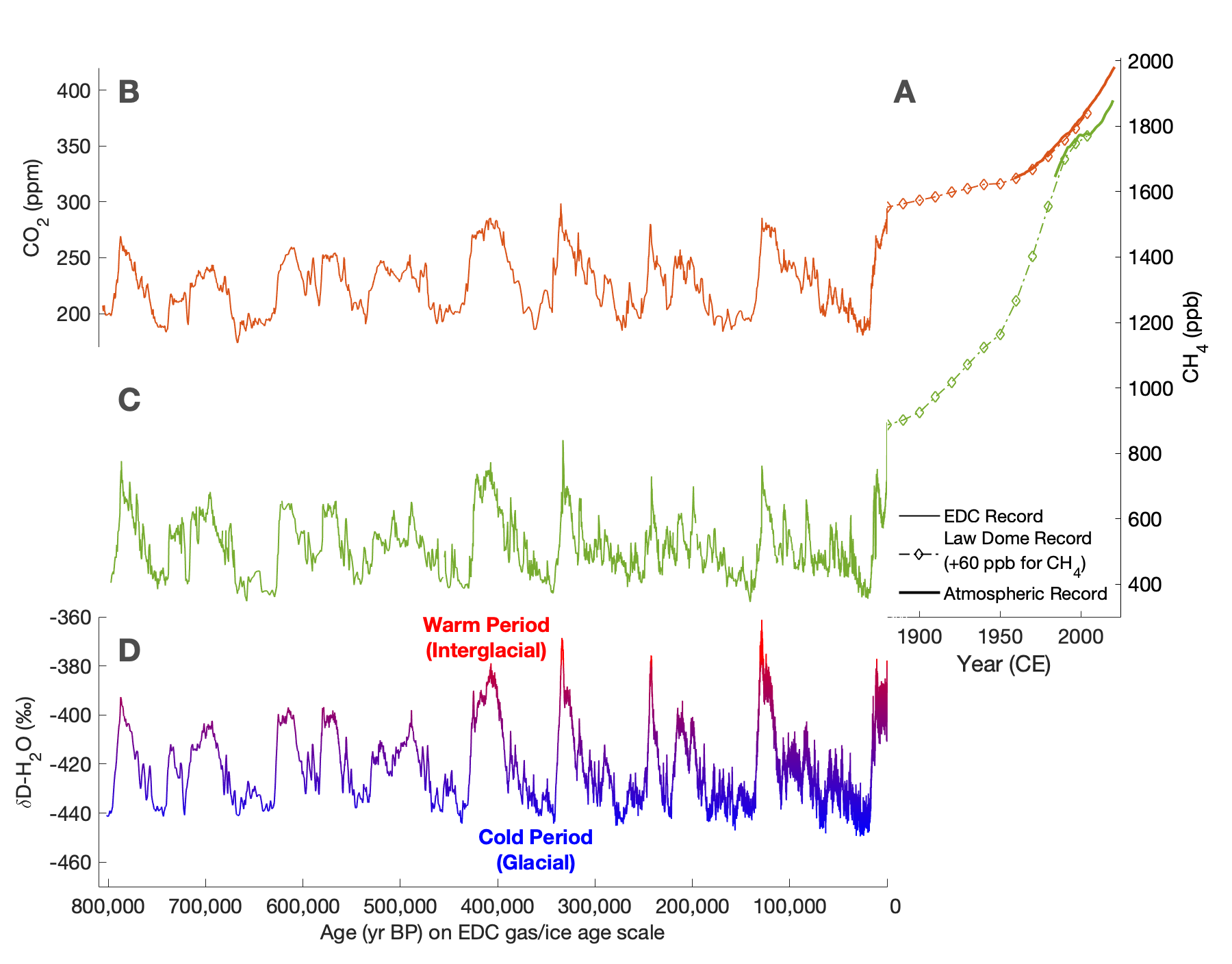
The fidelity of ice-core air as a record of past atmospheres is confirmed by the precise agreement between ice-core-derived records of GHGs and instrumental records over the last 40–60 years (Fig. 1a; Macfarling Meure et al. 2006). Ice cores from Antarctica have provided 800,000-year-long records of major GHGs in high resolution (CO2, CH4), covering eight complete glacial–interglacial cycles, with recent efforts aimed at recovering ice, and subsequently atmospheric composition, up to several million years old (Dahl-Jensen 2018). These data confirm that the modern atmospheric concentrations of GHGs and their rates of increase are unprecedented in at least the last 800,000 years.
Ice-core CO2 records have established the fundamental relationship between atmospheric CO2 and climate (derived from stable isotopes of H2O in the ice surrounding the bubbles, which are temperature proxies; Wendt et al. p. 102) on glacial–interglacial timescales (Fig. 1a, c; Jouzel et al. 2007). GHG records on centennial and millennial timescales provide strong evidence of abrupt changes to Earth's climate system and atmosphere. For example, ice-core CH4 records from Greenland and Antarctica reveal dramatic variability on decadal timescales that coincides with similarly abrupt Northern Hemisphere climate changes recorded in Greenland ice cores, highlighting the sensitivity of CH4 to abrupt climate change (Chappellaz et al. 1993).
 |
|
Figure 1: (A) CH4 and CO2 records from the Law Dome ice core (Macfarling Meure et al. 2006; dot/dashed lines) and the global mean atmospheric records (Hofman et al. 2006; solid lines) from 1875 to 2020 CE. In the modern atmosphere, Antarctic CH4 is roughly 60 ppb lower than the atmospheric mean CH4 because CH4 sources are concentrated in the Northern Hemisphere. To account for this, the Law Dome CH4 record was increased by 60 ppb. (B–D) 800,000 year Antarctic records of (B) CO2, (C) CH4, and (D) δD-H2O, a proxy for temperature, all from the EPICA Dome C (EDC) ice core (Jouzel et al. 2007). |
Measurements of the stable and radioactive isotopic composition of atmospheric GHGs can reveal which sources contributed to changes in concentration over time. Because major GHG sources often have distinguishable isotopic compositions, variability in the strength of these sources over time had measurable impacts on the past atmospheric isotopic signature. Recently, the suite of trace gas measurements made on ice-core samples has expanded to include these isotope measurements, providing valuable constraints on the causes of past GHG variability and the complex dynamics of Earth's climate system. For example, records of stable isotopes in CO2 suggest that land-based CO2 sources caused abrupt CO2 rises during the last deglaciation (20,000-10,000 years ago), while ocean-based sources were responsible for a more gradual rise (Bauska et al. 2016). Records of CH4 isotopes strongly suggest that changes in microbial sources, rather than abrupt releases of geologic CH4, dominated the deglacial CH4 change (Dyonisius et al. 2020).
Modern records of anthropogenic change
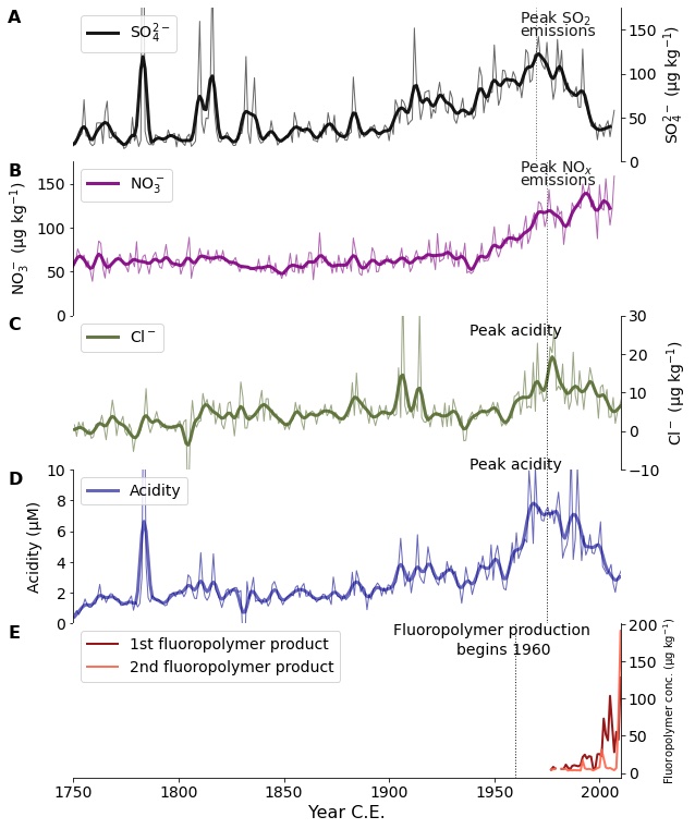
Ice cores preserve changes in atmospheric chemistry and pollution over human history (Wensman et al. p. 108). For example, they record how atmospheric sulfate, which causes acid rain and influences global climate, tripled between 1900 and 1980 due to fossil-fuel burning, and then declined from 1980 to present day following clean-air policies in North America and Europe (Mayewski et al. 1986; Fig. 2a). They also show how atmospheric nitrate concentrations have doubled since the 1950s due to increased NO and NO2 (collectively NOX) emissions from fossil-fuel combustion and agriculture, which have changed the biogeochemical cycling of nitrogen since the pre-industrial era (Hastings et al. 2009; Fig. 2b).
Ice cores also provide information about the past and current abundance of atmospheric oxidants, which are chemicals that react with air pollutants (e.g. SO2) and hydrocarbons (e.g. CH4), yielding products that can cool (e.g. SO4) or warm (e.g. CO2 the atmosphere. These reactions can determine the lifetime of GHGs such as CH4, so investigating how oxidants have changed can help estimate the warming potential of GHGs at different times in Earth's history. Although many oxidants such as ozone and the hydroxyl radical are too chemically reactive to be recorded in ice-core gas bubbles, proxies for these oxidants can indicate how oxidants have varied in the past. For example, clumped oxygen isotopes (i.e. 18O18O instead of 16O16O or 16O18O) constrain how ozone concentrations increased in the 20th century due to industrialization (Yeung et al. 2019).
 |
|
Figure 2: Recent measurements of dissolved ice-core species that tell us about atmospheric chemistry and pollution. Thin colored lines show annual measurements and bolded lines show multiyear averages. These ice cores are from the Greenland Ice Sheet and the Canadian Arctic. (A) Summit sulfate from Cole-Dai et al. (2013); (B) Summit nitrate from Geng et al. (2014); (C) Tunu chloride from Zhai et al. (2021); (D) Tunu acidity from Zhai et al. (2021); and (E) Devon Ice Cap and Mt. Oxford (northern Canada) perfluoroalkyl carboxylic acids from Pickard et al. (2020). |
Atmospheric halogens (elements including chlorine, bromine, and iodine) are some of the most reactive oxidants in the atmosphere and influence important species such as sulfate, volatile organic compounds, mercury, and ozone. It is difficult to know how atmospheric halogens have varied because measurements of reactive halogens have only been possible in the past few decades, but ice-core records combined with models can provide insight into how atmospheric halogen chemistry has changed due to anthropogenic pollution. For example, ice-core records of chlorine excess (i.e. chlorine that comes from a source other than sea salt; Fig. 2d) show how chlorine is correlated with atmospheric acidity (Fig. 2e) since the preindustrial, and atmospheric models indicate this correlation is due to acidity reacting with sea-salt aerosols (Zhai et al. 2021).
Ice cores also record pollutants that only exist due to anthropogenic activities. Figure 2e shows ice-core concentrations of perfluoroalkyl carboxylic acids, which are byproducts of refrigerants that have been found in ice cores starting in the mid-20th century and increasing rapidly after 1990 (Pickard et al. 2020). Records of these pollutants, along with concentrations of short-lived species such as sulfate, nitrate, and halogens, show how profoundly human activities have affected the chemistry and composition of the atmosphere, especially in the past 100 years.
Conclusions
Ice-core records provide unique archives of past changes in atmospheric composition and chemistry due to natural and anthropogenic causes. Ice-core gas records have provided information about past GHG concentrations and their relationship with global climate on glacial–interglacial and millennial timescales, as well as unprecedented increases in GHGs over the last century due to fossil-fuel burning. Analyses of major ions and other non-gaseous compounds have improved our understanding of anthropogenic pollution and its influence on atmospheric chemistry and climate. As older ice-core records are recovered and measurement techniques continue to improve, so too will our knowledge of past atmospheric composition and its interaction with climate and chemistry—knowledge that is essential for understanding the modern climate system and predicting future change.
affiliationS
1Department of Earth, Environmental and Planetary Sciences, Rice University, Houston, TX, USA
2College of Earth, Ocean, and Atmospheric Sciences, Oregon State University, Corvallis, USA
3Department of Atmospheric Sciences, University of Washington, Seattle, USA
contact
Asmita Banerjee: Asmita.Banerjee@rice.edu
Ben Riddell-Young: riddellb@oregonstate.edu
Ursula Jongebloed: ujongebl@uw.edu
references
Bauska TK et al. (2016) Proc Natl Acad Sci USA 113: 3465-3470
Chappellaz J et al. (1993) Nature 366: 443-445
Cole-Dai J et al. (2013) J Geophys Res Atmos 118: 7459-7466
Dahl-Jensen D (2018) Nat Geosci 11: 703-704
Dyonisius MN et al. (2020) Science 367: 907-910
Geng L et al. (2014) Proc Natl Acad Sci USA 111: 5808-5812
Hastings MG et al. (2009) Science 324: 1288
Hofman DJ et al. (2006) Tellus B 58: 614-619
Jouzel J et al. (2007) Science 317: 793-796
Macfarling Meure C et al. (2006) Geophys Res Lett 33: L14810
Mayewski PA et al. (1986) Science 232: 975-977
Pickard HM et al. (2020) Geophys Res Lett 47: e2020GL087535
Kathleen A. Wendt1, H.I. Bennett2, A.J. Carter3 and J.C. Marks Peterson1
Ice cores provide a unique window into Earth's climate history. This article explores the various climate indicators stored in ice cores and some of the scientific insights that have resulted from studying them.
Climate indicators
Ice cores contain an invaluable record of Earth's past climate. The climate information stored in ice cores, or climate indicators, can be broadly divided into three categories: (1) atmospheric composition, (2) regional atmospheric circulation, and (3) local temperature and snowfall. Past atmospheric composition is determined by directly sampling ancient air which was trapped during the transformation of snow to ice (McCrimmon et al. p. 112). As overburdened snow layers compact, the interconnected pores within old snow (firn) close and trap atmospheric gases (e.g. O2, N2, Ar, CO2, CH4) within the newly formed bubbles (Banerjee et al. p. 104). Analyzing the isotopes of atmospheric gases provides insight into their potential sources and sinks.
Past changes in regional atmospheric circulation (i.e. transport pathways) are inferred by examining mineral dust, volcanic ash, and ions in ice cores. The distribution of dust grain size indicates transport strength, and the geochemical composition of dust and ash reveals potential source areas. Dust concentrations can also provide insight into global aridity, while variations in ions (e.g. Na+, Cl-, Ca2+, Mg2+, NH4+) and organic compounds are used to infer regional changes, such as sea-ice extent and marine productivity.
Past changes in local air temperature are inferred from the analysis of oxygen (δ18O) and hydrogen (δD = δ2H) stable isotope ratios in the water molecules of ice. Air temperatures influence the degree of mass fractionation of water isotopes during the vapor condensation process inside clouds. Isotopic ratios of δ18O and δD are translated to past temperatures using an empirical relationship derived from, for example, a spatial network of modern snowfall analysis or temperature–depth profiles within the ice sheet. During periods of rapid warming, a vertical temperature gradient within the porous firn column can form, causing gases to thermally fractionate. As a result, deviations in 15N/14N and 40Ar/36Ar provide an additional proxy for rapid temperature changes. Changes in temperature and snowfall accumulation influences the rate of ice formation, which provides further information about local climate conditions.
Long-term climate change
In the 1960s, glaciologists at Byrd Station (Antarctica) drilled an ice core that dated back to the last glacial period (Martin et al. p. 100). Their pioneering work revealed that cooler temperatures during the last glaciation coincided with lower greenhouse gas concentrations (Berner et al. 1980). This discovery led to a fundamental understanding of the link between global temperature and greenhouse gas concentrations.
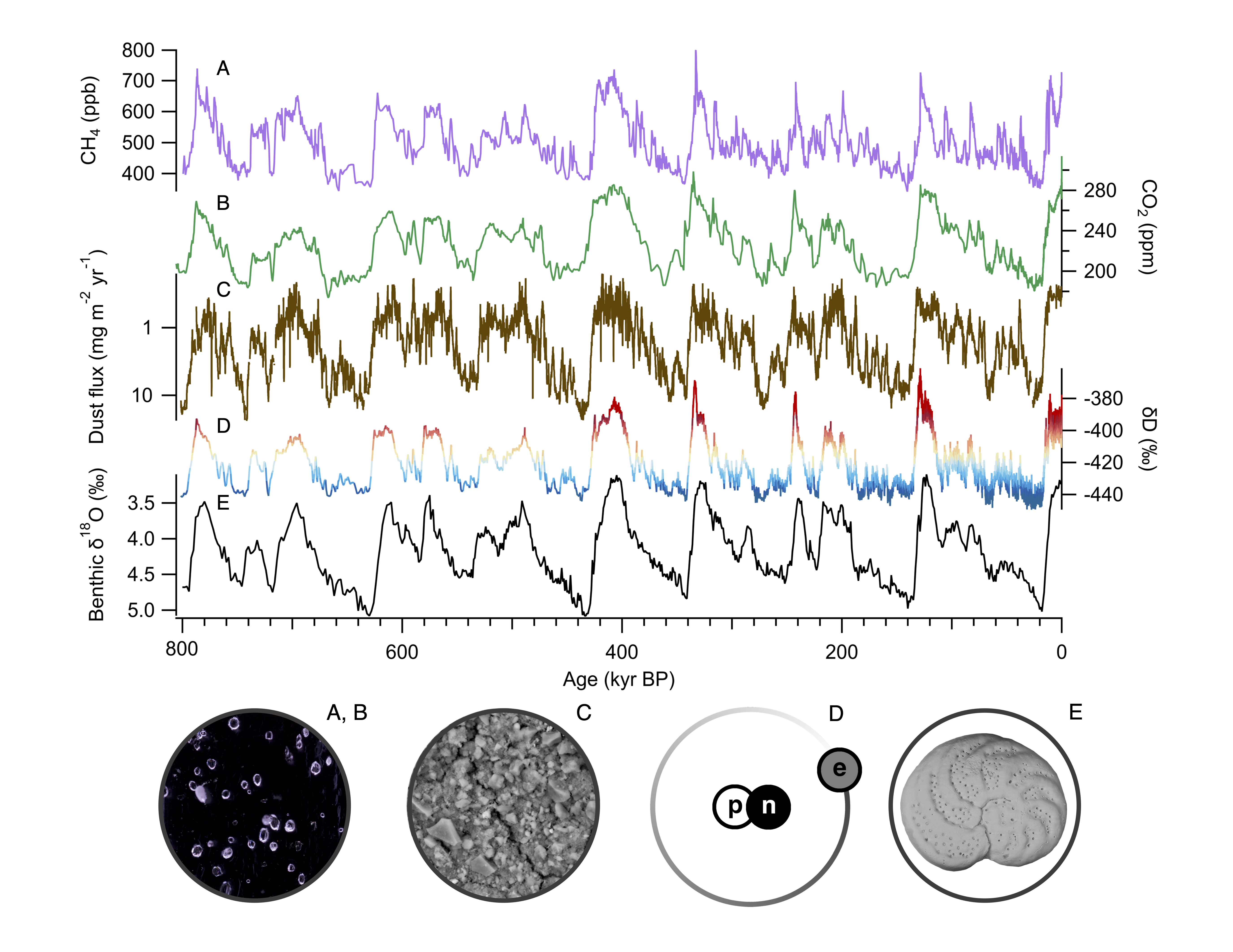
Over the last five decades, a multinational effort to collect several deep ice cores from the East Antarctic Plateau has resulted in the now iconic 800-thousand-year (kyr) climate record (Fig. 1). The compiled record offers a window into past greenhouse gas concentrations, Antarctic temperatures, and atmospheric transport properties over the last eight glacial cycles. Climate indicators within the ice reveal major synchronous variations on glacial–interglacial timescales (Fig. 1). The recorded variations resemble the blade of a jagged saw with the troughs representing glacial periods. When compared to warm interglacial periods, glacials are characterized by cooler Antarctic temperatures, lower greenhouse gas concentrations, and dustier winds blowing over Antarctica (Fig. 1a-d). For example, Antarctic temperatures were between 4 and 10℃ cooler (e.g. Buizert et al. 2021) and atmospheric CO2 concentrations were over 100 ppm lower (Lüthi et al. 2008) during the Last Glacial Maximum (20 kyr ago) relative to pre-industrial conditions.
 |
|
Figure 1: Climate indicators in Antarctic ice (A-D) and marine sediments (E) reveal climate change over the last 800 kyr. From top: (A-B) Atmospheric methane (purple, Loulergue et al. 2008) and carbon dioxide (green, Bereiter et al. 2015); (C) 250-year smoothed dust flux plotted on a reversed logarithmic scale (brown, Lambert et al. 2012); (D) Variations in δD (rainbow, Jouzel et al. 2007) which reflect Antarctic temperatures (red indicating warmer and blue indicating cooler); and (E) Variations in the δ18O of benthic foraminifera in marine sediments (black, Lisiecki and Raymo 2005). |
The 800-kyr ice-core record shows remarkable similarities to other paleoclimate records worldwide. Most notable is the δ18O of benthic foraminifera in deep ocean sediments (Fig. 1e), which is widely used as an index for global ice volume (Lisiecki and Raymo 2005; Christ et al. p. 116). Examining synchronous variations provides a complete picture of the global changes that occur on glacial–interglacial timescales and, most importantly, what drives them. The study of ice cores and other long-term climate records have contributed to the understanding that glacial cycles are paced by Earth's orbital configuration. Climate changes caused by variations in incoming solar radiation are further amplified by a cascade of feedbacks within the climate system. This is best observed during a glacial termination, when climate records worldwide show a systematic and rapid transition to interglacial conditions (Fig. 1). Ice cores have been instrumental in revealing the order, timing, and magnitude of these key climate shifts.
Abrupt climate change
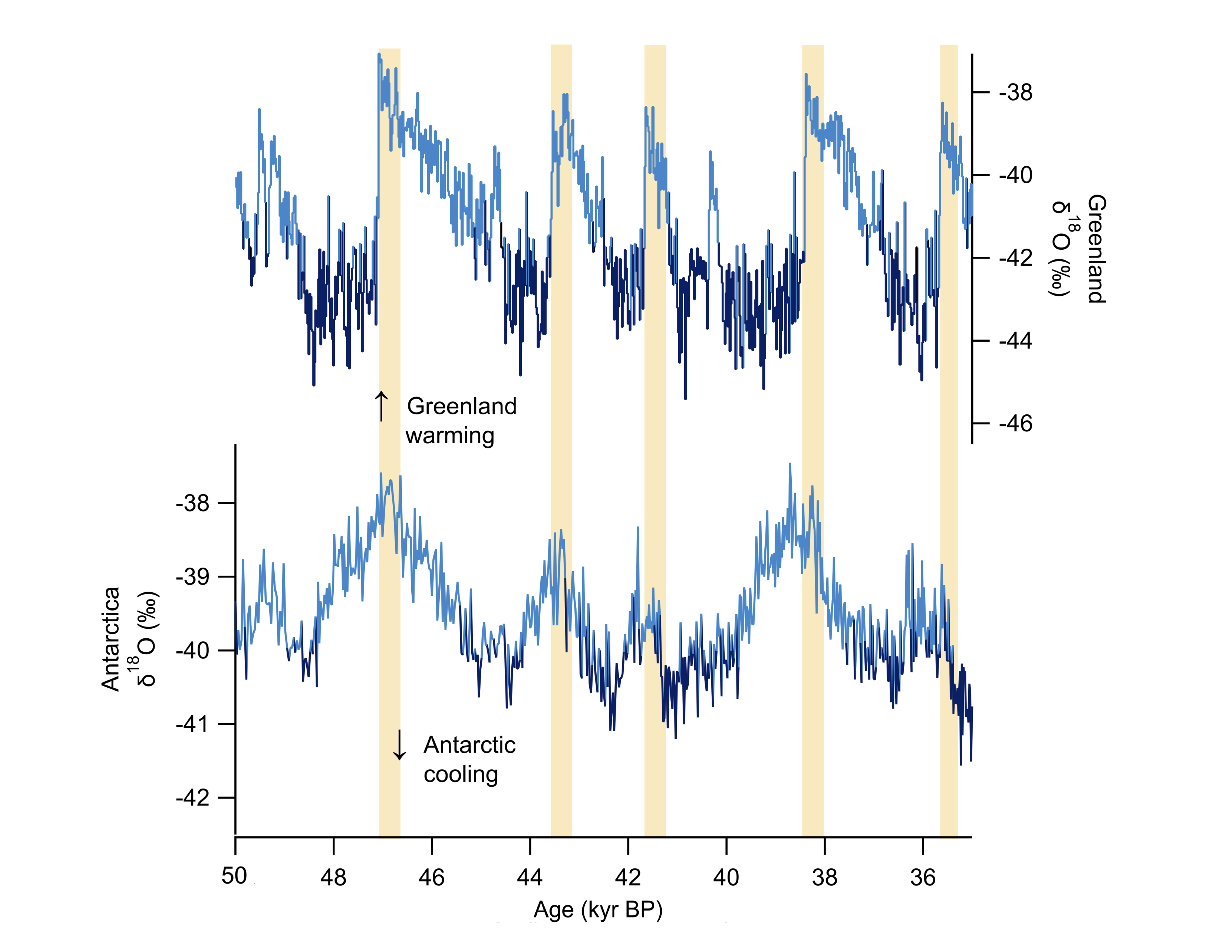
Ice cores also provide unique insight into past periods of abrupt climate change (Alley 2000). Evidence from ice cores suggests that Greenland experienced large swings in temperatures at millennial-scale intervals throughout the last glaciation (Fig. 2; Dansgaard et al. 1993). Abrupt warming periods, known as Dansgaard-Oeschger (D-O) events, are defined by a ~10°C increase in Greenland temperatures over the short period of a few decades (Severinghaus and Brook 1999). Approximately 200 years after an abrupt warming in Greenland, Antarctic temperatures begin to cool (WAIS Divide Project Members 2015; Fig. 2). Similarly, abrupt cooling in Greenland ultimately gives way to Antarctic warming. This phenomenon is known as the thermal bipolar seesaw (Stocker and Johnsen 2003). It can be explained by perturbations in the northward heat transport via the Atlantic Ocean, which exert opposite temperature effects on both hemispheres. The 200-year delay in Antarctic temperatures is the result of a north-to-south propagation of the climate signal through oceanic processes that operate on centennial timescales.
Recent work on high-resolution Antarctic ice cores have revealed variations in CH4, CO2, and the relationship between δ18O and δD that are near-synchronous with Northern Hemisphere D-O events (e.g. Bauska et al. 2021). The timing of these coeval changes suggests a rapid atmospheric response that is uncoupled from ocean circulation. Shifts in the distribution of tropical precipitation or the meridional position of midlatitude westerlies could rapidly propagate signals between hemispheres. These interhemispheric mechanisms are the focus of ongoing research. Resolving these finer-scale changes shed important light on fast-acting feedbacks within Earth's climate system.
 |
|
Figure 2: Example of abrupt climate change during the last glacial period. Top panel shows ice δ18O from North Greenland (NGRIP Members 2004) plotted on the adjusted GICC05 chronology. Bottom panel shows ice δ18O from West Antarctica (WAIS Divide Project Members 2015) plotted on the WD2014 chronology. Yellow bars indicate the timing of D-O events, during which Greenland warms rapidly. Shades of blue illustrate how relatively cold atmospheric temperatures were at each location, with darker blues showing colder temperatures. |
Climate sensitivity
Ice cores support our understanding of past climatic changes and play a critical role in future climate projections. Since Eunice Foote's discovery of CO2's warming properties in 1856 (Foote 1856), the study of greenhouse gases and their influence on Earth's radiative balance has remained a cornerstone of climate sciences. The study of past atmospheric greenhouse gas concentrations drastically improved our understanding of their role in amplifying climate changes that result from variations in incoming solar radiation due to rhythms in Earth's orbit. For example, approximately 40% of the radiative forcing associated with the last glacial termination has been attributed to changes in atmospheric CO2 and CH4 (Lorius et al. 1990). Greenhouse gas records from ice cores can also be used in conjunction with reconstructions of global temperature to quantify equilibrium climate sensitivity (i.e. the magnitude of temperature change associated with a given change in greenhouse gas concentration). Future climate projections that aim to quantify the global temperature response to fossil-fuel emissions require accurate estimates of climate sensitivity. If not for the ancient atmosphere encapsulated in ice cores, predicting future climate change would be far more uncertain.
affiliationS
1College of Earth, Ocean, and Atmospheric Sciences, Oregon State University, Corvallis, USA
2Institute of Arctic and Alpine Research, University of Colorado Boulder, USA
3Scripps Institution of Oceanography, University of California, San Diego, USA
contact
Kathleen A. Wendt: kathleen.wendt@oregonstate.edu
references
Alley RB (2000) Proc Natl Acad Sci USA 97: 1331-1334
Bauska TK et al. (2021) Nature 14: 91-96
Bereiter B et al. (2015) Geophys Res Lett 42: 542-549
Berner W et al. (1980) Radiocarbon 22: 227-235
Buizert C et al. (2021) Science 372: 1097-1101
Dansgaard W et al. (1993) Nature 364: 218-220
Foote E (1856) Am J Sci Arts 22: 382-383
Jouzel J et al. (2007) Science 317: 793-796
Lambert F et al. (2012) Clim Past 8: 609-623
Lisiecki LE, Raymo ME (2005) Paleoceanography 20: PA1003
Lorius C et al. (1990) Nature 347: 139-145
Loulergue L et al. (2008) Nature 453: 383-386
Lüthi D et al. (2008) Nature 453: 379-382
North Greenland Ice Core Project Members (2004) Nature 431: 147-151
Severinghaus JP, Brook EJ (1999) Science 286: 930-934
Kaden C. Martin![]() 1, S. Barnett2, T.J. Fudge3 and M.E. Helmick
1, S. Barnett2, T.J. Fudge3 and M.E. Helmick![]() 4,5
4,5
The depth–age relationship of an ice core is critical to its interpretation; it constrains rates of change and allows for comparisons among records. Chronology advancements will be critical to the investigation of new ice cores over the coming decades.
Ice cores provide remarkable insight into past environmental change. As snow falls on glaciers and ice sheets, it traps things like past air, dust, volcanic ash, and soot from fires (Wendt et al. p. 102; Banerjee et al. p. 104; Brugger et al. p. 106). These environmental indicators are preserved in the ice sheet as fresh snow falls on the surface. By drilling down into an ice sheet or glacier (Davidge et al. p. 98), researchers can travel back in time to determine what the climate was like when the snow fell. However, placing these environmental indicators into a global climate context critically relies on our ability to date these ancient layers.
To better understand the time held within ice, ice-core scientists create chronologies. A chronology defines the relationship between time and depth in ice. Like counting tree rings, physically distinct layers and chemical impurities in ice correlate to seasons. These layers are well preserved as an ice sheet grows, aiding in the production of highly-resolved and well-constrained chronologies. To create the time–depth relationship, ice-core scientists rely on a range of techniques including measurements of distinct layers, comparisons with other well-dated records, physics models of snow compression and ice flow, and radiometric dating.
Chronology fundamentals
An intuitive method to develop an ice chronology is via annual-layer counting, where seasonally varying compounds or properties of ice can be used to identify yearly cycles (Fig. 1). Water isotopes, dust, and conductivity are commonly used to achieve this (Andersen et al. 2006; Sigl et al. 2016). Physical properties of ice also aid in this stratigraphy, such as visually distinct winter and summer layers due to extreme polar seasons. Annual layers become thinner with depth due to large-scale ice flow, reducing temporal resolution. Deep within an ice sheet, just a few meters can contain thousands of years of snowfall. Here, other techniques must be used as annual layers become indiscernible and dating becomes challenging.
 |
|
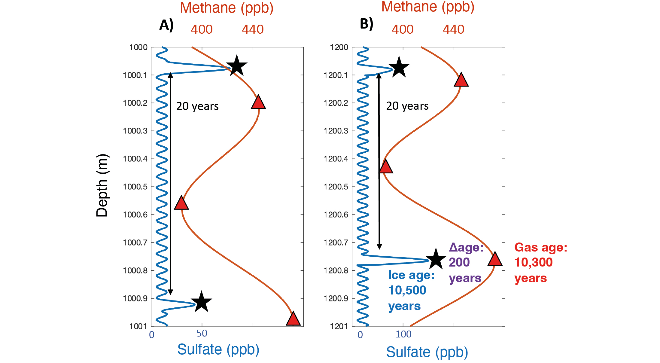
Figure 1: (A, B) Two idealized ice-core records, showing annual layers and volcanic events of sulfate in ice (blue) and methane concentrations in gas (orange). Annual cycles of sulfate can be counted to produce an ice chronology, while methane features can be dated using a firn model reconstruction of Δage or by examining abrupt events. The ages of cores A and B are synchronized by volcanic signals (black stars) and methane features (red triangles). Δage can be calculated between distinct features, and is 200 years in (B). |
Chronological information can be shared between cores by matching evidence of abrupt geological events. During volcanic eruptions, ash and sulfate can be deposited onto the ice sheets. These distinct layers are then preserved in the ice. If the same layer is found in different ice cores, the age of that layer can be transferred between them (Fig. 1a, b). This technique has been used to synchronize the ice chronologies of cores from Greenland and Antarctica at these discrete tie-points (Seierstad et al. 2014; Svensson et al. 2020).
A unique challenge of ice-core chronologies is that the ice crystals and the air bubbles trapped between them have different ages. Near the surface, air can move through spaces between grains of snow. This movement of air stops at the snow–ice transition, at ~40–120 m depth (McCrimmon et al. p. 112). At this point, pathways for air have closed and bubbles are sealed in ice, becoming isolated from the atmosphere. Therefore, the ice is older than the gases trapped within. This means that two chronologies are needed—one to study the ice, and one to study the gases.
The age difference between ice and gas at the same depth is Δage ("delta age"). This age difference is not the same everywhere, nor is it constant for a given core. This is because Δage responds to changes in how fast snow turns into ice, which is set by local temperature and snowfall rate (Schwander et al. 1997).
As trapped air is younger than the ice surrounding it, dating gases requires different techniques. Because Δage is the ice–gas age difference, Δage and ice chronologies can be utilized to produce gas chronologies. Δage is accurately estimated during abrupt climate change events due to distinct features that occur in environmental indicators of both gas and ice (Buizert et al. 2015). During time periods without abrupt events, Δage is estimated by modeling the physics of snow compression, emulating how snow turns into ice given the climatic conditions at the time. Estimated and modeled Δages alongside annual-layer-counted ice chronologies are then used to calculate the gas chronology. Gas chronologies are also often dated using methane (CH4). Due to rapid atmospheric mixing of CH4, its atmospheric concentration is similar everywhere in Earth's lower atmosphere at any given time. This means that changes in one core can be matched to the same change in another core (Blunier and Brook 2001). This allows for the most accurate gas chronology to be transferred to any ice core (Fig. 1b, c).
As the array of well-dated ice cores and chronological information increases, data inversion techniques can be used to establish tie-points between different cores and bring their chronologies into agreement (Lemieux-Dudon et al. 2010). Such projects have successfully supported Antarctic chronologies (Parrenin et al. 2015). The key to data inversion is to utilize all available age constraints, like volcanic events, CH4 matches, and annual-layer counts, in a mathematical framework. The framework then calculates a chronology that is within the bounds of the uncertainties and physical properties of the available data. This is a powerful technique, as it can overcome shortcomings of individual methods and reduce the time needed to construct new chronologies for recently recovered cores.
Dating the oldest ice
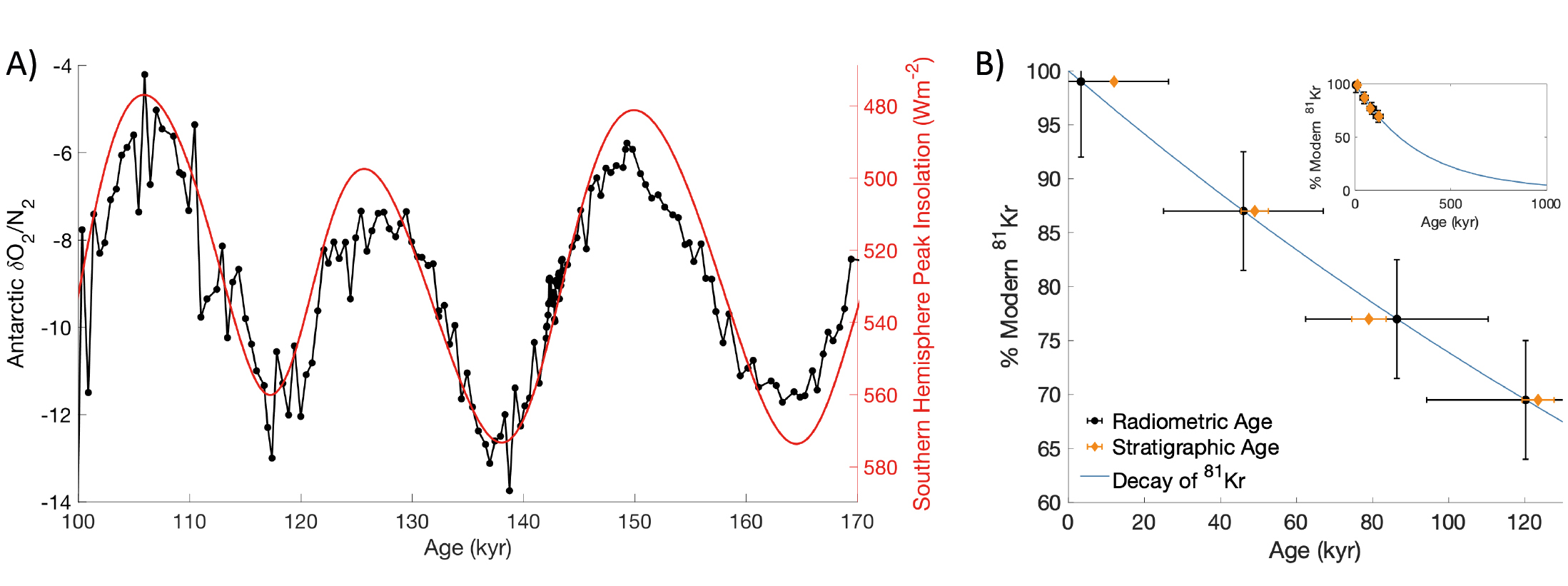
The oldest continuous ice-core records, found primarily in the East Antarctic Ice Sheet, have been dated by orbital tuning. This technique is necessary where annual layers become indistinguishable. Orbital tuning utilizes the known relationship between a proxy, like δO2/N2, and the cyclical variation of sunlight due to Earth's orbital cycles (Fig. 2; Oyabu et al. 2021). This method has been widely applied to marine sediment cores, where the variations in oxygen isotopes can be linked to changes in solar insolation and ice volume (Imbrie and Imbrie 1980).
 |
|
Figure 2: (A) The oxygen-to-nitrogen ratio (δO2/N2, black; Oyabu et al. 2021), measured from the Dome Fuji Ice Core in East Antarctica, and Southern Hemisphere peak summer sunlight, or insolation (red, note reverse axis; Laskar et al. 2004). The snow–ice transformation rate influences the δO2/N2, and this process correlates well with the location's amount of summer sunlight. By comparing δO2/N2 to past sunlight, age can be approximated. (B) Decay rate of 81Kr (blue), and the comparison between conventional dating techniques (orange) and measurements of 81Kr (black; Buizert et al. 2014). Inset: Same as in (B), but scaled to cover this technique's effective range. |
Another technique for dating old ice utilizes radiometric dating, where the known decay rate of radioactive isotopes in preserved bubbles can be used to determine when they were isolated from the atmosphere. Two useful radioisotopes are Argon-40 (40Ar) and Krypton-81 (81Kr). 81Kr is produced in the atmosphere by cosmic-ray interactions with the stable isotopes of Kr. As the atmospheric concentration of 81Kr has been relatively constant over the last 1.5 million years, a measurement of an old sample will be less than the modern concentration due to radiometric decay. The difference in concentration between an old and modern sample is set by the decay rate of 81Kr, and can be used to determine when the gas in the sample was trapped in the ice. The half-life of 81Kr is 229 kyr BP, providing a dating range of 0.5 to 1.5 million years—useful when dating old ice (Fig. 2). Ar isotopes in ice cores record the decay and outgassing of radioactive potassium in the mantle, which provides a unique chronologic marker (Bender et al. 2008).
Outlook
Chronologies are critical to placing ice-core records into a global context, enabling direct comparisons between natural greenhouse-gas variations and records of environmental change in other archives. Chronology development is an ever-growing field, supported by advancements in instrumentation, new chemical measurements, and mathematical models as past cores are updated and new projects are planned. Techniques for absolute dating are being developed to support deep ice-core projects targeting continuous climate records of 1.5 million years, such as the new COLDEX and BeyondEPICA projects, and discontinuous climate records from blue-ice areas, like Allan Hills, Antarctica (Kehrl et al. 2018).
affiliations
1College of Earth, Ocean, and Atmospheric Sciences, Oregon State University, Corvallis, USA2School of Earth and Sustainability, Northern Arizona University, Flagstaff, USA
3Department of Earth and Space Science, University of Washington, Seattle, USA
4School of Earth and Climate Science, University of Maine, Orono, USA
5Climate Change Institute, University of Maine, Orono, USA
contact
Kaden C. Martin: martkade@oregonstate.edu
references
Andersen KK et al. (2006) Quat Sci Rev 25: 3246-3257
Bender ML et al. (2008) Proc Natl Acad Sci USA 105: 8232-8237
Blunier T, Brook EJ (2001) Science 291: 109-112
Buizert C et al. (2014) Proc Natl Acad Sci USA 111: 6876-6881
Buizert C et al. (2015) Clim Past 11: 153-173
Imbrie J, Imbrie JZ (1980) Science 207: 943-953
Kehrl L et al. (2018) Geophys Res Lett 45: 4096-4104
Laskar J et al. (2004) Astron Astrophys 428: 261-285
Lemieux-Dudon B et al. (2010) Quat Sci Rev 29: 8-20
Oyabu I et al. (2021) Cryosphere 15: 5529-5555
Parrenin F et al. (2015) Geosci Model Dev 8: 1473-1492
Schwander J et al. (1997) J Geophys Res Atmos 102: 19,483-19,493
Seierstad IK et al. (2014) Quat Sci Rev 106: 29-46
Lindsey Davidge![]() 1, H.L. Brooks
1, H.L. Brooks![]() 2 and M.L. Mah
2 and M.L. Mah![]() 3
3
Polar and alpine glacial ice is scientifically valuable, but it is logistically challenging to drill, transport, and store. We summarize the process of retrieving and analyzing a new core and identify archived samples that might be available for new research.
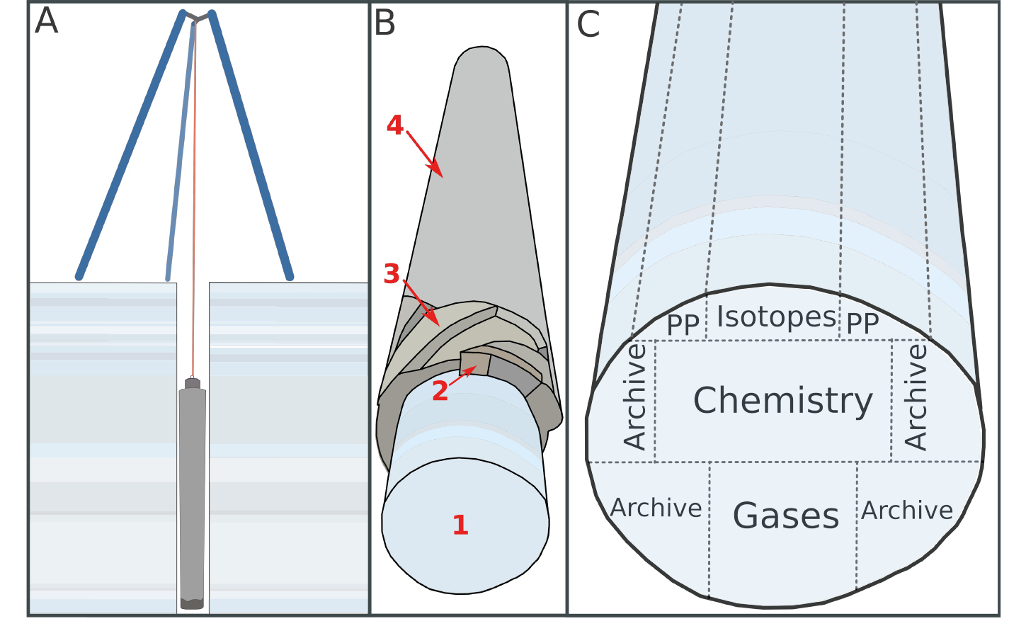
Ice cores collected from polar ice sheets and alpine glaciers provide a frozen archive of past atmospheric gases and precipitation that are important to glaciological and climate sciences. Ice-core analyses produce exceptionally well-resolved observations of local, regional, or global changes in the atmosphere over time. This is because as snow falls, a variety of physical processes affect its material properties and composition, and these signals get preserved through time. For example, ice flow direction affects the mineral orientation of frozen water, atmospheric composition determines the particle load and aqueous chemistry of an ice layer, and global and regional temperatures change the isotopic composition of the precipitation falling at an ice-core site; further, atmospheric gases trapped in the pore spaces between ice crystals are preserved and can be measured directly from ice-core samples (Banerjee et al. p. 104). Consequently, there are dozens of analyses that may be desirable to perform on a single ice-core sample. Drilling and preserving ice-core samples is challenging because cores are retrieved from frozen, often remote, and sometimes very deep (i.e. thousands of meters) sites. Despite this, cores are routinely recovered from scientifically advantageous locations, and ice samples are typically archived in storage facilities, where they may be available to support future research.
 |
|
Figure 1: (A) Simplified cross section of an ice-drilling operation (not to scale). (B) Stylized drawing of an electromechanical drill, showing the retrieved core (1), cutters (2), helical flights (3), and core barrel (4). (C) An example of a cut diagram used to specify the target analyses for each portion of the core (PP = physical properties). |
Drilling an ice core
Though the ice drilling process is similar at most sites, scientific objectives dictate the desired ice volume and depth, and cargo restrictions and site temperature may constrain equipment choices. Most core segments are about 10 cm in diameter and 1 m long, though the exact dimensions are determined by the size of the drill. Most core samples are retrieved by electromechanical drills; these drills contain a hollow cylinder, called the core barrel, that is equipped with rotational cutting teeth at the bottom (see Johnsen et al. 2007). Above the core barrel, an anti-torque device stabilizes the drill within the borehole while the cutters are spinning, and the entire drill assembly is suspended from a tripod or tower by an armored electrical cable (Fig. 1a). The rotating cutters pulverize a ring of ice, leaving a cylindrical pillar intact to enter the core barrel, while the remnant ice chips are removed from the cutting interface by circulating fluid and/or by helical flights (Fig. 1b). Each time the drill has progressed far enough to fill the core barrel, the ice pillar is broken off at its base, and the entire assembly is winched up to the surface. For electromechanical drills, the cutting force is supplied by electric motors, and the rate of penetration can be controlled by changing the weight above the bit. When drilling in ice warmer than -10ºC, mechanical cutters tend to stick, and ice chip transport becomes difficult; at such sites, a ring-shaped heater is typically used to incise the ice instead in a process called thermal drilling (see Zagorodnov and Thompson 2014).
Glaciers and ice sheets are particularly inhospitable drilling environments. At the surface, heavy winds scour and redistribute recent snowfall, often burying scientific equipment or causing large snow drifts. Deeper in the ice sheet, ice flows under its own weight, causing deep boreholes to deform and close over time. Choices about infrastructure and equipment typically balance labor and cargo requirements with drilling efficiency and core quality. For example, drilling within covered trenches is the best way to avoid the impacts of drifting snow and bad weather, but a windscreen or tent might be a preferred alternative at sites where cargo capacity is limited or where the planned drilling season is short. Small drills or hand augers are used in alpine environments, where transporting personnel, equipment, and cores is often done by small aircrafts or even by foot or pack animal (Matoba et al. 2014; Schwikowski et al. 2014). However, deep ice-drilling projects in Greenland and Antarctica—which must penetrate multiple kilometers into the ice sheet—can utilize longer drill barrels, longer and stronger winch cables, and taller towers to minimize the number of trips up the borehole and accelerate the field campaign (Bentley and Koci 2007; Zhang et al. 2014). Boreholes deeper than about 300 m need to be backfilled with drilling fluid to prevent the borehole from collapsing (Talalay et al. 2014), though drilling fluid can also contaminate fractures within the core, which limits possible analyses.
Field storage and transportation
Once at the surface, cores are labeled with orientation and depth information and packaged carefully for transportation. Ice-core samples are susceptible to breakage, alteration, and melt, which means that preserving cores in the field and during transportation requires significant preparation; deep ice cores can be particularly fragile as they are removed from the ice sheet and rapidly decompress at the surface (Neff 2014). To inhibit physical, chemical, and biological alteration, it is desirable to store core samples at temperatures that are comparable to the in-situ temperature of the ice or at a maximum of about -20ºC. Cores are typically placed in insulated shipping boxes for protection during field storage and transportation. At polar drilling sites that remain frozen at the surface year-round, a shallow, covered trench dug into the snow is often enough to insulate the boxed cores for months or years. Storage at alpine glacier sites can be more complicated because these sites tend to be warmer and wetter than polar locations (e.g. Tsushima et al. 2021). Because of this, drilling at alpine sites is often seasonally constrained, and it is important to remove cores from these temperate sites as quickly as possible and place them in freezer storage.
The availability of onsite storage and field access limitations determine the method and frequency of transportation. Because ice cores from many polar sites can be safely stored at the drilling location—and because polar sites are often accessed by fixed-wing aircraft with substantial capacity for cargo—there is typically less urgency around transporting these cores, and their transportation can be scheduled similarly to other field-site cargo (e.g. Slawny et al. 2014). These cores are sometimes moved into temporary freezer storage at permanent research stations before being shipped to their destination country in refrigerated shipping containers aboard cargo ships or in smaller refrigerators aboard large aircrafts. For ground transport, temperature-controlled containers are transported by truck to national archive facilities or university laboratories for analysis.
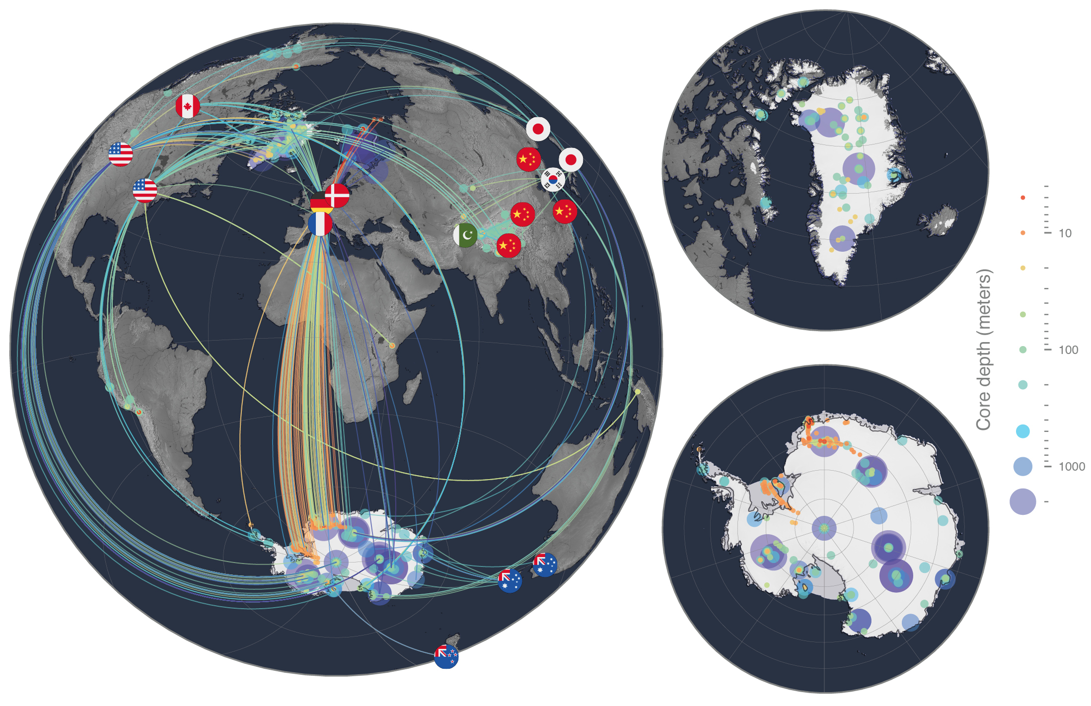 |
|
Figure 2: Map of selected ice drilling sites and storage locations, including details of Greenland (top right) and Antarctica (bottom right). Lines link the drill site and ice-storage location for each core (left). Many other archived samples exist in repository facilities around the world. Complete details are available in a corresponding database (Davidge et al. 2022). |
Distribution and analysis of ice-core samples
Obtaining diverse measurements on an ice core typically requires that core samples be partitioned and distributed to multiple laboratories (Fig. 1c; as in Souney et al. 2014). Core samples are processed in one of two ways: discretely, by cutting the ice into small pieces and measuring the average properties of each subsample; or continuously, by melting one-meter "sticks" of the core from top to bottom and analyzing the resulting melt stream. It is desirable to make continuous measurements from ice-core samples when possible, because this method produces high-resolution timeseries while also minimizing sample handling and the potential for contamination (e.g. Osterberg et al. 2006; Röthlisberger et al. 2000). The volume of ice that is sent to each collaborating laboratory depends on analytical method requirements and project objectives.
Long-term ice-core storage
Notably, a portion of many cores has been archived in long-term storage facilities for use by future investigators. Ice from hundreds of field sites is stored in ice-core repositories within national research centers or universities (Hinkley 2003). Many of these samples are available for future research – and, indeed, many ice-core studies were conceptualized long after the ice core was originally retrieved. We provide a map of selected ice archives in Figure 2. Many core samples can be accessed by contacting the repository and proposing new strategies to leverage existing core samples to answer outstanding research questions.
affiliationS
1Department of Earth and Space Science, University of Washington, Seattle, USA
2School of Earth and Climate Sciences & Climate Change Institute, University of Maine, Orono, USA
3Department of Electrical and Computer Engineering, University of Minnesota, Minneapolis, USA
contact
Lindsey Davidge: ldavidge@uw.edu
references
Bentley CR, Koci BR (2007) Ann Glaciol 47: 1-9
Davidge L et al. (2022) Zenodo, doi:10.5281/zenodo.7076469
Johnsen SJ et al. (2007) Ann Glaciol 47: 89-98
Matoba S et al. (2014) Ann Glaciol 55: 83-87
Neff PD (2014) Ann Glaciol 55: 72-82
Osterberg EC et al. (2006) Environ Sci Technol 40: 3355-3361
Röthlisberger R et al. (2000) Environ Sci Technol 34: 338-342
Schwikowski M et al. (2014) Ann Glaciol 55: 131-136
Slawny KR et al. (2014) Ann Glaciol 55: 147-155
Souney JM et al. (2014) Ann Glaciol 55: 15-26
Talalay P et al. (2014) Cold Reg Sci Technol 98: 47-54
Tsushima A et al. (2021) Ann Glaciol 62: 353-359
Jessica Badgeley![]() 1, T.J. Fudge1, B. Koffman
1, T.J. Fudge1, B. Koffman![]() 2 and S. Rupper
2 and S. Rupper![]() 3
3
Ice cores have changed the way we understand the Earth. Ice cores drilled in the 1990s in Greenland showed definitively for the first time the abrupt nature of climate change events in the past (e.g. Dansgaard et al. 1993; Grootes et al. 1993). Ice cores from Antarctica have yielded a continuous climate history of the past 800,000 years, as well as snapshots of climate older than two million years (Jouzel et al. 2007; Yan et al. 2019, Bergelin et al. 2022), providing important context for climate changes underway today. The global network of ice cores drilled in remote mountainous and polar regions provides insight into topics beyond climate, including the history of wildfires and anthropogenic activities (e.g. Dahe et al. 2002; Grieman et al. 2018). Today, we continue to drill ice cores in Greenland, Antarctica, and mountain glaciers worldwide to better understand the Earth.
It takes a global community of scientists from a variety of disciplines to locate sites, drill cores, conduct analyses, and interpret the data in the broader context of the Earth system (Fig. 1). Like many countries around the world, the United States (US) recognizes both the contributions of ice-core science and the importance of a dedicated and inclusive scientific community. In 2022, the US National Science Foundation, via the Ice Drilling Program, funded a workshop for US early-career researchers to become more deeply involved in the ice-core community. This opportunity came together as the Ice Core Early Career Workshop (ICECReW; icedrill.org/meetings/ice-core-early-career-researchers-workshop-icecrew). Participants shared a collective desire to develop resources to help communicate ice-core science to undergraduate students and ice-core-adjacent researchers, inspiring this contribution to Past Global Changes Magazine.
The following 10 articles resulted from collaborations among the early-career scientists who attended the ICECReW workshop. The first article follows an ice core from the field to the lab. The next article addresses how to build an ice-core timescale, which is essential for placing measurements in context. The following eight articles cover key areas of ice-core science and adjacent fields: climate, atmosphere, wildfires, human activity, microbes, snow-to-ice transition, sub-ice materials, and sea-level change.
 |
|
Figure 1: Photos highlight key elements of ice-core research, from geophysical surveys of potential drilling locations to laboratory analysis and timeseries data: (A) Glacier survey on Denali, Alaska (Photo credit: Brad Markle); (B) Radar echogram from West Hercules Dome, Antarctica (Image credit: T.J. Fudge); (C) Ice-core drilling rig on Mount Logan, Canada (Photo credit: Brad Markle); (D) Ice-core barrel at WAIS Divide, Antarctica (Photo credit: Brad Markle); (E) Ice core from the Juneau Ice Field, Alaska (Photo credit: Brad Markle); (F) Ice-core transport by Basler aircraft at Byrd Station, Antarctica (Photo credit: Lora Koenig); (G) US National Science Foundation Ice Core Facility, Colorado (Photo credit: NSF-ICF); (H) Processing samples in the Pico-Trace Ultraclean Lab, Lamont-Doherty Earth Observatory of Columbia University, New York, USA (Photo credit: Bess Koffman); (I) Ice-core thin section (Photo credit: British Library); (J) Ice-core CO2 and isotope data from the EPICA Dome C ice core, Antarctica (Jouzel et al. 2007; Lüthi et al. 2008; Parkinson 2016) |
In reflecting on the important advances of the past decade, one thing is clear. Our community is stronger – and the science is better – when everyone is included. Inclusion has been particularly challenging during the COVID-19 pandemic, and one goal of ICECReW was to connect US early-career researchers of all races, genders, identities, abilities, and disciplines. Inclusion must occur at every level – for instance, the International Partnerships in Ice Core Sciences (IPICS; pastglobalchanges.org/ipics) open science meetings foster international inclusion. Through both individual and institutional actions, we can create a community where all feel welcome.
In addition to building a more inclusive ice-core community, continued advances in ice-core science will be enabled through measurements of ice from new sites. Some current and future projects include multiple searches for a continuous climate record spanning 1.5 million years in East Antarctica, and projects targeting previous warm periods—such as the Last Interglacial (~130,000 years ago)—to determine the amount and rate of sea-level rise at that time. New cores from mountain regions are filling in the global network and providing important regional perspectives. In the coming decades, ice coring will not only expand on Earth but will also likely extend to the Moon and Mars. These are all significant undertakings that require international partnership and cooperation.
Analytical improvements and integration of ice-core data with other proxy records and with models will be just as important for the field as drilling new cores. Clumped isotope analysis enables insight into past atmospheric conditions, while micrometer-scale measurements push the spatial and temporal resolution of the old, highly-thinned portions of ice cores. Advances in timescale development already permit synchronization of ice cores with many paleoclimate proxy records, allowing for global assimilation with climate models. Such efforts provide benchmarks for model performance, aiding in our projections of future climate change.
As we look to the future of ice-core science, we see great promise among the current generation of early-career scientists. We are excited to showcase their perspectives on some of the important ice-core science developments in the articles that follow.
affiliationS
1Department of Earth and Space Sciences, University of Washington, Seattle, USA
2Department of Geology, Colby College, Waterville, ME, USA
3Department of Geography, University of Utah, Salt Lake City, USA
contact
Bess Koffman: bkoffman@colby.edu
references
Bergelin M et al. (2022) Cryosphere 16: 2793-2817
Dahe Q et al. (2002) Ann Glaciol 35: 278-284
Dansgaard W et al. (1993) Nature 364: 218-220
Grieman MM et al. (2018) Clim Past 14: 637-651
Grootes PM et al. (1993) Nature 366: 552-554
Jouzel J et al. (2007) Science 317: 793-797
Lüthi D et al. (2008) Nature 453: 379-382
Parkinson A (2016) Doctoral Thesis, University of Cambridge, doi:10.17863/CAM.6321
Anne de Vernal and Claude Hillaire-Marcel
Following the summer insolation peak triggering the present interglacial, the Arctic Ocean shelves experienced seasonal sea ice, whereas the central basin remained mostly perennially ice-covered. During the Quaternary, sub-perennial sea ice persisted, with short summer ice-free windows during the warmer interglacials.
Perennial vs. seasonal sea ice
Sea ice plays an important role in the climate system, not only because of the ice–ocean–albedo feedback, but also because it is a freshwater reservoir that modifies the ocean stratification when it forms or melts. From this viewpoint, the presence of perennial vs. seasonal sea-ice cover is particularly critical. The perennial sea ice that survives from one year to another has a relatively simple role in regional- to basin-scale climate and ocean conditions: it is thick (>3 meters), moves slowly, maintains high albedo through the summer season, and restricts exchanges of energy and gas at the ocean–atmosphere interface (Fig. 1). Presently, the west central Arctic Ocean is the only place where perennial sea ice maintains year after year (Fig. 2).
Seasonal sea ice is more complex and more elusive, as it melts in summer, following variable patterns and time windows. This results in a sea-ice extent varying from year to year and from one region to another (e.g. Chen et al. 2016). Thus, sea-ice extent experiences large amplitude and high frequency (interannual to interdecadal) changes related to atmospheric (Cai et al. 2021) and hydrographic (e.g. Ricker et al. 2021; Belter et al. 2021) patterns. Beyond the direct impact on sea-surface temperature through a reduced albedo, the summer sea-ice melting lowers the sea-surface salinity and enhances the stratification of upper water masses, which in turn fosters freezing and sea-ice formation with the atmospheric cooling during the following fall–winter seasons.
Furthermore, seasonal, first-year sea ice is thinner than multiyear ice. It moves at a higher speed along ocean currents and is thus more efficiently exported (Kwok et al. 2013). Hence seasonal sea ice is a highly dynamic component of the Arctic climate. In addition, its export from the Arctic Ocean into the North Atlantic, via the western Fram Strait, impacts the Atlantic Meridional Overturning Circulation (AMOC). As it is a source of freshwater, it enhances the stratification of the subarctic North Atlantic and thus may lead to reduced convection. However, the winter freezing of the low salinity surface waters leads to brine production and vertical mixing. Hence, the vertical convection that occurs close to the seasonal sea-ice edge plays a role in deep water formation, which implies that shifts in the limits of winter sea ice impact the locus and strength of AMOC turning points (Bretones et al. 2022).
For all the reasons summarized above, seasonal sea ice is a critical climate parameter, but it is an elusive one, due to its high variability in time and space.
Evidence for seasonal Arctic sea ice in the early–middle Holocene
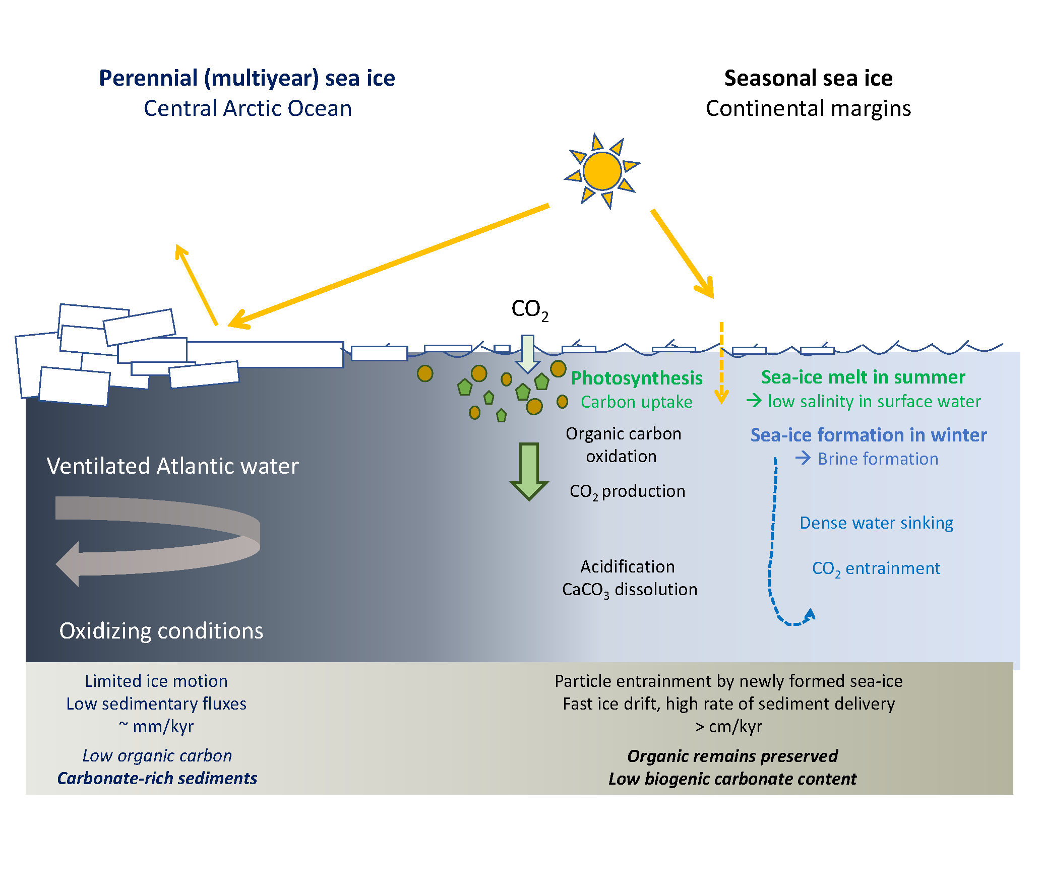 |
|
Figure 1: Sketch of oceanic, environmental and sedimentary processes under perennial and seasonal sea ice. Modified from de Vernal et al. (2020). |
Sea-ice environments characterized by open seawater conditions in summer experience high primary productivity of phototrophic organisms (such as diatoms and dinoflagellates). There are several types of biological remains providing indications of summer sea-ice-free conditions. They include microfossils and molecular biomarkers related to primary producers (de Vernal et al. 2013a), which permit the documentation of seasonal sea ice based on the analyses of sediment.
Sedimentary sequences from Arctic shelves of the Chukchi, East Siberian, Laptev, and Kara seas provide evidence for relatively high productivity under open summer sea-ice conditions, during the middle Holocene, from about 8000 to 4000 years ago (de Vernal et al. 2013b; Hörner et al. 2016; Stein et al. 2017). Some of the records show enhancement of sea ice during the late Holocene, which has lasted until the ongoing recent warming that has led to sea-ice decline.
In the central Arctic Ocean, sedimentation rates are very low, on the order of centimeters per thousand years or less (de Vernal et al. 2020; Hillaire-Marcel et al. 2017), precluding the establishment of high temporal-resolution records. Furthermore, the low organic carbon content of the sediment is accompanied by scarce primary productivity indicators. Nonetheless, relatively high concentrations of dinoflagellate cysts in early–middle Holocene sediment from the southeastern Lomonosov Ridge provide evidence for phototrophic productivity and episodic seasonal ice-free conditions off the Laptev Sea. In comparison, barren sediments from the polar and western sectors of the Lomonosov Ridge suggest that perennial sea ice prevailed throughout the whole Holocene (de Vernal et al. 2020). Such data provide evidence of a dipole pattern in sea-ice distribution during the early–middle Holocene, as seen in recent years, notably in 2007, 2012, and 2019 (Yadav et al. 2020; Fig. 2).
Assessing perennial vs. seasonal sea ice in the central Arctic Ocean from biological remains
Perennial sea ice is difficult to assess because it is based on negative evidence that relies on the absence of any indication for phototrophic, sea-ice-free productivity. Barren pelagic/hemipelagic sediments could be interpreted as indicative of perennial sea ice. However, cold water phototrophic taxa belong mostly to diatoms or dinoflagellates that yield organic biomarkers and/or microfossil remains made of biogenic silica (diatoms) or organic matter (dinoflagellate cysts), which do not necessarily preserve well. The undersaturation of the water column in silica prevents the preservation of diatoms down to the seafloor. Moreover, the subduction and circulation of North Atlantic waters in the Arctic Ocean, below the perennial ice cover, may cause oxidation of organic material, especially in the context of low sedimentation rates and high exposure to oxidizing conditions. As a result of low organic carbon fluxes, and low sedimentation rates, the sediments that blanket the floor of the perennially ice-covered Arctic Ocean are poor in organic carbon but rich in biogenic carbonates (Fig. 1). Hence, the surface sediments of the Arctic Ocean are often characterized by a rich carbonate fauna on the seafloor but are almost barren in organic remains that might have witnessed past phototrophic production (de Vernal et al. 2020).
The only positive indication of permanent sea ice that possibly exists is indirect: it comes from an ostracod species, Acetabulostoma arcticum, which lives as a parasite of a nematode occupying brine channels in multiyear sea ice (Cronin et al. 2012). This ostracod was present in the Amerasian Basin, western Arctic, for the last 400,000 years, including during the interglacial stages, which leads us to consider Arctic sea ice as a perennial feature since at least 400,000 years ago (Cronin et al. 2012).
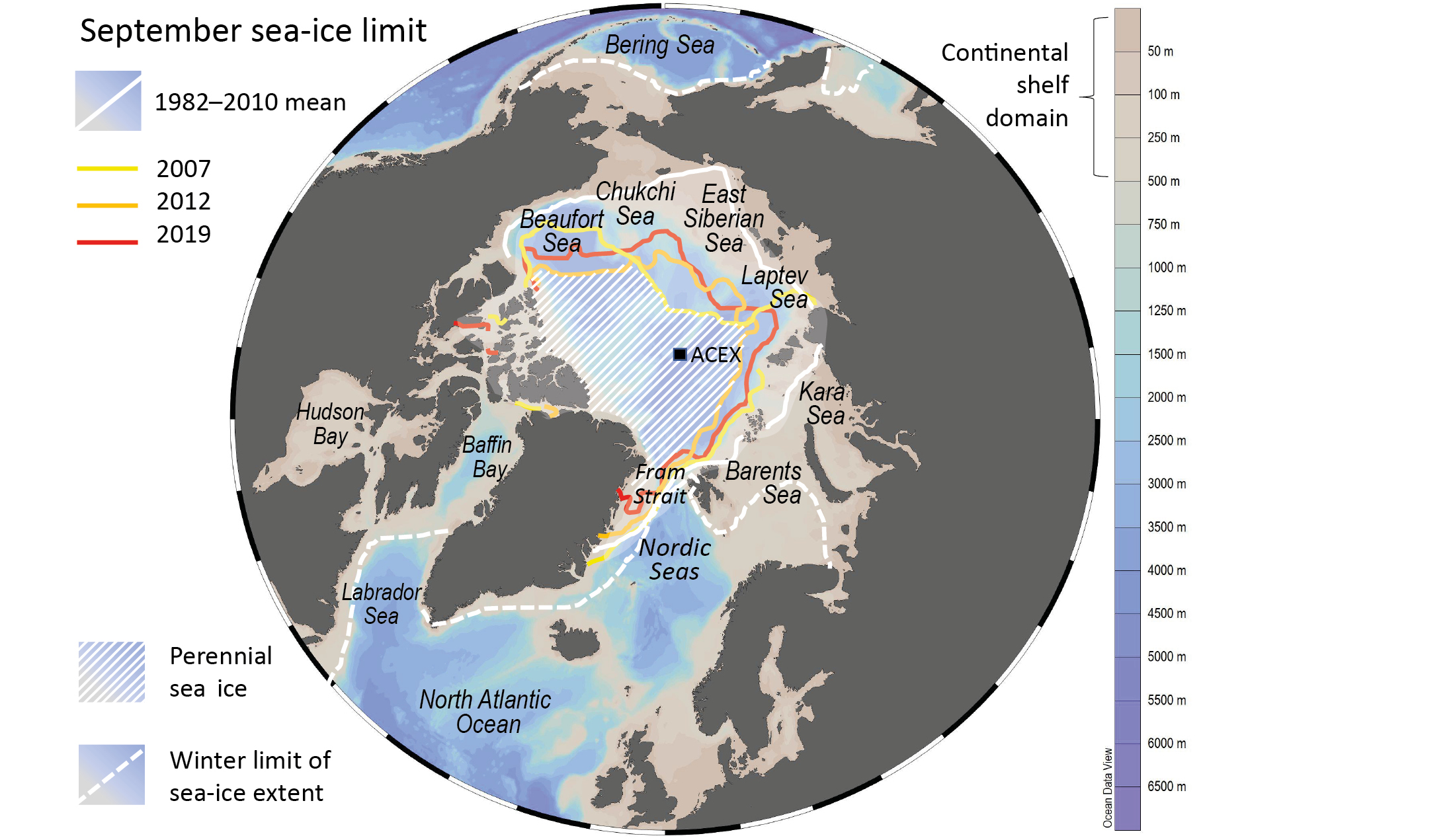 |
|
Figure 2: Map of the Arctic Ocean showing recent limits of minimum sea-ice extent in September (from Yadav et al. 2020), which might correspond to those of the mid-Holocene, and location of the Arctic Coring Expedition (ACEX) drilling site mentioned in the text. Evidence of early–middle Holocene seasonal sea ice was reported for the Chukchi, East Siberian, and Laptev seas (e.g. de Vernal et al. 2013b; Hörner et al. 2016; Stein et al. 2017). |
The 2004 Arctic Coring Expedition (ecord.org/expedition302), during which long sequences near the North Pole were drilled (Fig. 2), may shed some light on the history of the Arctic sea ice. The record of organic-walled dinoflagellate cyst that may document phototrophic conditions revealed almost barren assemblages in the upper sequence encompassing the last two million years, suggesting perennial sea ice over the central Arctic Ocean throughout most of the Quaternary (Matthiessen et al. 2018).
Shifting from perennial to seasonal Arctic-wide sea-ice cover
Unraveling the long-term history of the Arctic sea ice is challenging. Sedimentary records from shelves yield biogenic material that allows us to document past sea ice from proxies, but only for the interval that followed the submergence of shelves accompanying the global sea-level rise of the last deglaciation. Sedimentary records from the deep basin yield older but equivocal proxy records, not to mention issues about their chronology (Hillaire-Marcel et al. 2017). Nevertheless, all data available converge toward perennial sea ice over the central Arctic basin during most, if not all, of the Quaternary. A positive indication for seasonal sea-ice openings during the early–middle Holocene transition, at least sporadically, exists for the southeastern sector of the Arctic Ocean (de Vernal et al. 2020), when summer insolation was still near its maximum. Other short-lived intervals with seasonally open water possibly occurred during earlier insolation maximums, but this is still not well documented. On the contrary, indirect evidence from ostracods suggests a resilient perennial sea-ice cover in the western Arctic, at least during the last three interglacials (Cronin et al. 2012). Hence, the evidence points to resilient perennial sea ice in the central Arctic Ocean during the Quaternary, perhaps interrupted by yet poorly documented short time windows of regional summer ice-free conditions. On geologic (pre-Anthropocene) timescales, the shift from seasonal to quasi-permanent perennial sea ice probably occurred before the Pleistocene. In that context, the recent trend toward seasonal sea ice over a large part of the Arctic Ocean is exceptional, with unavoidable consequences on the climate–ocean system.
affiliation
Geotop, University of Quebec in Montreal, Canada
contact
Anne de Vernal: devernal.anne@uqam.ca
references
Belter HJ et al. (2021) Cryosphere 15: 2575-2591
Bretones A et al. (2022) J Climate 35: 109-124
Cai Q et al. (2021) J Clim 34: 9931-9955
Chen HW et al. (2016) J Geophys Res Atmos 121: 14,433-14,455
Cronin TM et al. (2012) Nat Geosci 5: 631-634
de Vernal A et al. (2013a) Quat Sci Rev 79: 1-8
de Vernal A et al. (2013b) Quat Sci Rev 79: 111-121
de Vernal A et al. (2020) Proc Natl Acad Sci USA 117: 26,069-26,075
Hillaire-Marcel C et al. (2017) Geochem Geophys Geosyst 18: 4573-4585
Hörner T et al. (2016) Quat Sci Rev 143: 133-149
Kwok R et al. (2013) J Geophys Res Oceans 118: 2408-2425
Matthiessen J et al. (2018) Quat Sci Rev 192: 1-26
Ricker R et al. (2021) J Clim 34: 5215-5227