PAGES Magazine articles
Marie Sicard![]() 1,2, A.M. de Boer1,2 and L.C. Sime3
1,2, A.M. de Boer1,2 and L.C. Sime3
The 16 models that simulated the Last Interglacial climate as part of the CMIP6/PMIP4 exercise consistently produce a smaller Arctic summer sea-ice area compared to the pre-industrial period, but their reduction ranges widely (28–96% of the pre-industrial area). Causes for these differences need further investigation.
Why are we interested in changes in the Arctic sea ice during the Last Interglacial?
The Last Interglacial (LIG, 129-116 kyr before present (BP)) is characterized by a strong insolation forcing leading to an Arctic land summer warming of 4–5°C relative to the pre-industrial period (PI; Guarino et al. 2020). The increase in surface temperatures has been associated with changes in Arctic sea ice potentially comparable in magnitude to those projected for the near future (Guarino et al. 2020). Simulations of the LIG climate, thus, provide a tool to study the processes and feedbacks related to current Arctic sea-ice loss and polar warming. The high availability of sea-ice proxy data, compared to previous interglacial periods, also makes the LIG a good case study to evaluate the ability of climate models to simulate sea ice during periods warmer than today. In recognition of the importance of the LIG in our understanding of climate change, it was formally included as a target period in the latest Paleoclimate Modelling Intercomparison Project (PMIP4). The joint experimental protocol differs primarily from the PI experiment in the astronomical parameters and greenhouse gas concentrations (Otto-Bliesner et al. 2017). The LIG PMIP4 experiment, thus, represents a reference point for discussions of model reconstruction of Arctic sea ice for this period.
What have we learned from the CMIP6/PMIP4 LIG experiment?
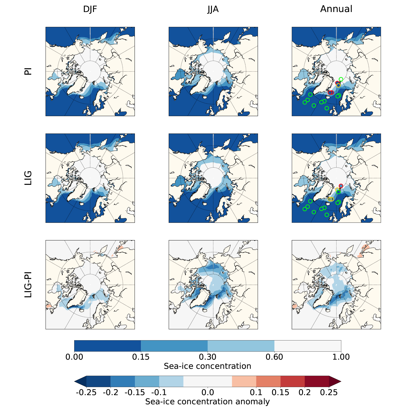
The Arctic sea ice, simulated by the 16 climate models that run the LIG experiment, was analyzed by Kageyama et al. (2021). Figure 1 shows the multi-model mean (MMM) for the winter (DJF), summer (JJA) and annual sea-ice concentration. The larger sea-ice retreat relative to the PI appears in summer when the insolation anomaly reaches its maximum. During this season, the Greenland, Barents and Chukchi seas experience the most significant ice loss. The minimum monthly MMM at the LIG is equal to 3.2 ± 1.5 × 10⁶ km2, which represents a decrease of about 50% compared to the PI. Three models (HadGEM3-GC3.1-LL, CESM2, and NESM3) simulate an above-average retreat of the sea-ice edge in summer relative to the PI, with a total sea-ice area close to, or less than, 1 × 10⁶ km2. However, of these three, only HadGEM3-GC3.1-LL and CESM2 have a realistic representation of the PI Arctic sea-ice seasonal cycle. The HadGEM3-GC3.1-LL model shows the largest sea-ice retreat, with the Arctic Ocean becoming ice-free at the end of summer (Guarino et al. 2020). On the other end of the spectrum, the INM-CM4-8, GISS-E2-1-G and FGOALS-g3 models simulate large sea-ice areas greater than 5 × 10⁶ km2 at the end of summer. This disparity between models is also found in winter. During this season, the maximum monthly MMM is equal to 16.0 ± 2.6 × 10⁶ km2, with most models simulating a slight increase compared to the PI. However, the ACCESS-ESM1-5, EC-Earth3-LR and INM-CM4-8 models show a reduced sea-ice area relative to the PI.
 |
|
Figure 1: Multi-model mean of the Arctic sea-ice concentration for the pre-industrial (PI) and Last Interglacial (LIG) periods and LIG-PI differences. Results are plotted for winter (DJF), summer (JJA) and the annual average. The fill color of the symbols corresponds to the observed values at sites where proxy data are available for the LIG (see Kageyama et al. (2021) for more details on the sea-ice data synthesis). For the PI, a dataset obtained from different satellite and in-situ observations is used (Reynolds et al. 2002). The color of the symbol outline indicates the number of models simulating the observed sea-ice cover: green for nine or more models, yellow for five to nine models and red for five or fewer models. Adapted from Kageyama et al. (2021). |
What is the cause of inter-model differences?
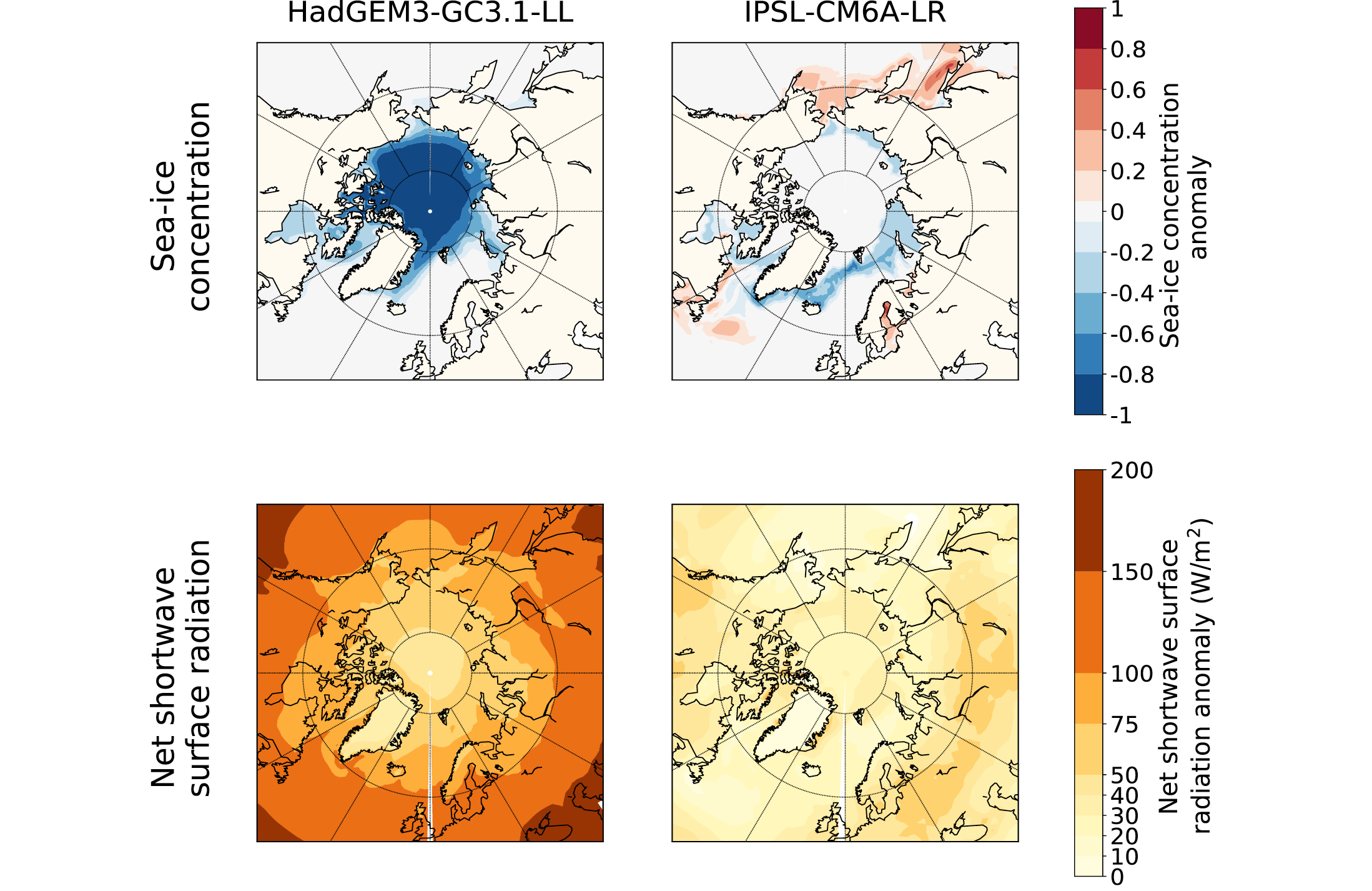
There are many characteristics of climate models that can lead to variable results, including differences in model physics and chemistry, discretization scheme and numerical resolution, parameterization of subgrid-scale processes, and tuning parameters. Given that these aspects of models and their feedbacks are interlinked non-linearly, it can be problematic to attribute specific differences in results to specific differences in process representation. However, some progress has been made. The large spread of sea-ice reduction in the PMIP4 models has been linked to differences in surface albedo and optical properties of clouds, which directly impact the surface radiation balance (Kageyama et al. 2021), as illustrated for the IPSL-CM6A-LR and HadGEM3-GC3.1-LL models in Figure 2.
An indepth analysis of processes explaining the LIG-PI difference in Arctic sea ice in the IPSL-CM6A-LR model highlighted the predominant influence of ice–air heat exchange on sea-ice melt, compared with ice–ocean heat exchange (Sicard et al. 2022). The specific sea-ice model formulation is also crucial. The large sea-ice loss in the HadGEM3-GC3.1-LL model has been attributed to the advanced melt-pond scheme included in its sea-ice model (Guarino et al. 2020). Specifically, the formation of melt ponds and leads allow the surface to absorb more incident solar radiation and, thereby, encourage more sea-ice melt (Diamond et al. 2021). Models with explicit representation of melt ponds seem to simulate particularly low LIG sea-ice area during summer (Diamond et al. 2021) and can also capture the summer warming observed in LIG continental records (Guarino et al. 2020).
Comparison with the new sea-ice data analysis
To allow for a model–data comparison, the PMIP4 synthesis paper on LIG Arctic sea ice includes an updated sea-ice data compilation (Malmierca-Vallet et al. 2018; Kageyama et al. 2021). This data synthesis is based on a set of marine records collected in the Arctic Ocean, Nordic seas, and northern North Atlantic. Models realistically capture annual sea-ice concentration in the North Atlantic region and the Norwegian Sea during the LIG, but generally simulate too much ice close to the sea-ice edge in the Greenland Sea and at the two northernmost sites in the central Arctic (Fig. 1). However, there are still significant uncertainties related to the sea-ice data in the central Arctic so that no strong conclusions can be drawn from it (Kageyama et al. 2021).
 |
|
Figure 2: Multi-model mean of the Arctic sea-ice concentration for the pre-industrial (PI) and Last Interglacial (LIG) periods and LIG-PI differences. Results are plotted for winter (DJF), summer (JJA) and the annual average. The fill color of the symbols corresponds to the observed values at sites where proxy data are available for the LIG (see Kageyama et al. (2021) for more details on the sea-ice data synthesis). For the PI, a dataset obtained from different satellite and in-situ observations is used (Reynolds et al. 2002). The color of the symbol outline indicates the number of models simulating the observed sea-ice cover: green for nine or more models, yellow for five to nine models and red for five or fewer models. Adapted from Kageyama et al. (2021). |
Conclusions and way forward
CMIP6 climate models that have run the LIG experiment all show a substantial reduction in the summer sea-ice area in the Arctic at 127 kyr BP (Kageyama et al. 2021). However, models disagree on the magnitude of this decline. Given the spread among model results and uncertainties in LIG Arctic proxy reconstructions of sea ice and temperature, it is therefore currently difficult to determine whether the Arctic Ocean experienced ice-free conditions during the LIG. Investigations so far have emphasized the importance of atmosphere–ice relevant processes, such as melt-pond formation or cloud optical properties, which are also crucial in determining radiation fluxes over sea ice (Guarino et al. 2020; Kageyama et al. 2021; Diamond et al. 2021; Sicard et al. 2022). Interestingly, ocean–ice fluxes have not yet been shown to be particularly significant, and have received less attention in the last few years compared to atmosphere–ice fluxes.
Ongoing work by the authors of this article and their groups aim to make further progress towards our understanding of LIG Arctic sea ice through several avenues. In a series of papers in preparation, we are investigating (1) the utility of proxies of LIG Arctic summer air temperatures to reconstruct sea ice (Sime et al. 2022); (2) the role of the LIG wind field, sea-ice transport, and Arctic ocean circulation in explaining reduced LIG sea ice (Sicard and de Boer, in prep); (3) the correspondence between LIG Arctic sea-ice loss, and that found in the CMIP6 transient simulation in which the atmospheric CO2 concentration increase at a rate of 1% per year (Eyring et al. 2016; Sicard and de Boer, in prep); and (4) the sensitivity of Arctic sea ice to the parameterization of meltponds for the LIG, and in the near future (Diamond et al. in prep).
Following the CMIP6/PMIP4 exercise, a flurry of papers has provided new insights on the state of the Arctic sea ice during the LIG, raising with them new and challenging scientific questions. With the targeted modeling studies, alongside ongoing work on sea-ice reconstructions, the future looks promising for further breakthroughs in our understanding of LIG Arctic sea ice, and how it relates to our future.
affiliations
1Department of Geological Sciences, Stockholm University, Sweden
2Bolin Centre for Climate Research, Stockholm University, Sweden
3British Antarctic Survey, Cambridge, UK
contact
Marie Sicard: marie.sicard@geo.su.se
references
Diamond R et al. (2021) Cryosphere 15: 5099–5114
Eyring V et al. (2016) Geosci Model Dev 9: 1937-1958
Guarino M-V et al. (2020) Nat Clim Chang 10: 928-932
Kageyama M et al. (2021) Clim Past 17: 37-62
Malmierca-Vallet I et al. (2018) Quat Sci Rev 198: 1-14
Otto-Bliesner BL et al. (2017) Geosci Model Dev 10: 3979-4003
Reynolds RW et al. (2002) J Clim 15: 1609-1625
Sicard M et al. (2022) Clim Past 18: 607-629
Sime LC et al. (2022) EGUsphere, doi:10.5194/egusphere-2022-594
Ruediger Stein![]() 1,2,3, A. Kremer3 and K. Fahl3
1,2,3, A. Kremer3 and K. Fahl3
Biomarker proxy records indicate that a permanent central Arctic Ocean sea-ice cover existed during the penultimate glacial (MIS 6) but was also still present during the Last Interglacial (MIS 5e), which was characterized by significantly warmer conditions than the present. However, extended seasonal open-water conditions occurred along the northern Svalbard–Barents Sea continental margin during MIS 5e.
Over the past three to four decades, coincident with global warming and atmospheric CO2 increase, Arctic sea ice has significantly decreased in its extent as well as in thickness (Kwok and Cunningham 2015; Notz and Stroeve 2016; 2018). The loss of sea ice results in a distinct decrease in albedo, causing further warming of ocean surface waters. When extrapolating this trend, the central Arctic Ocean might become ice-free during summers within about the next three to five decades, or even sooner (Masson-Delmotte et al. 2021). Based on a biomarker proxy reconstruction, such ice-free summers also occurred during the middle-late Miocene (12–6 million years before present (BP)), supported by climate modeling with simulated atmospheric CO2 concentrations of 450 ppm (Stein et al. 2016), a value we might reach in the near future. However, although the sea-ice conditions might be similar, the rate of change was quite different between both situations. Whereas the recent change from a permanent to a seasonal central Arctic Ocean sea-ice cover (strongly driven by anthropogenic forcing; cf. Notz and Stroeve 2016) proceeds over a few decades, the corresponding past (natural or non-anthropogenic) change occurred over thousands to millions of years. Furthermore, the closure of the Bering Strait, a shallow-water connection between the Arctic and Pacific oceans, also has an effect on sea-ice formation in the Arctic Ocean (Hu et al. 2015) that has to be considered when comparing past and present conditions.
Proxy-based reconstruction of past sea-ice conditions
One key aspect within the scientific and societal debate about present climate change is to distinguish and more precisely quantify natural and anthropogenic forcing of global climate change and related sea-ice decrease. In this context, it is fundamental to study paleoclimate records that document the natural climate, rates of change, and variability prior to anthropogenic influence. Paleoclimate reconstructions allow us to assess the sensitivity of the Earth's climate system to changes of different forcing parameters (e.g. CO2 and insolation; Fig. 1b) and boundary conditions (e.g. presence/absence of major ice sheets and opening/closure of ocean gateways), and to test the reliability of climate models by evaluating their simulations with boundary conditions very different from the modern climate. Of special interest are records representing past climatic conditions that were significantly warmer than the modern one, such as the early Eocene, mid-Miocene, and mid-Pliocene, as well as the Last Interglacial (LIG = Marine Isotope Stage (MIS) 5e), as these climate stages might represent analogs of our future climate, depending on the different IPCC scenarios and related future CO2 emissions (Burke et al. 2018; Masson-Delmotte et al. 2021).
 |
|
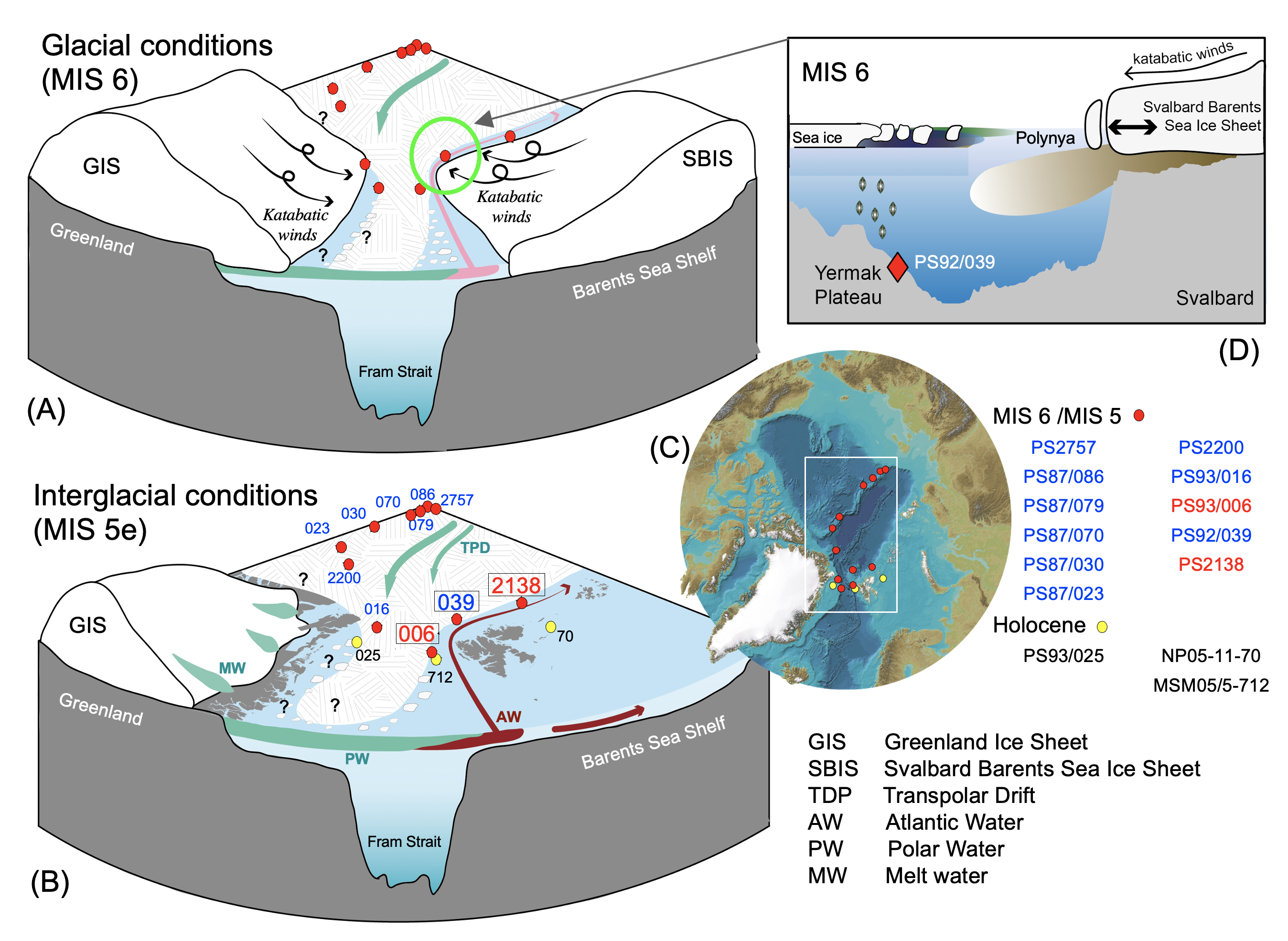
Figure 1: Changes in summer insolation, Arctic sea-ice cover and Svalbard–Barents Sea Ice Sheet extent during the last 200 kyr. (A) Modern mean September sea-ice concentration in the Fram Strait area and core locations; WSC (West Spitsbergen Current); EGC (East Greenland Current). (B) Summer insolation (Laskar et al. 2004). (C) Advance/retreat of Svalbard–Barents Sea Ice Sheet (Mangerud et al. 1998). (D) Strength of Atlantic water advection along the continental margin north of Svalbard (Wollenburg et al. 2001). (E) Biomarker proxy-based ("PIP25") reconstruction of sea-ice cover at cores PS92/039-2 and PS93/006-1; blue (red) circles indicate absence (presence) of alkenones at PS93/006-1 (Kremer et al. 2018). (F) PIP25 sea-ice record with (1) ice-free, (2) seasonal to ice-edge situation; and (3) extended to permanent sea-ice cover (Stein et al. 2017), and dinoflagellate records (i.e. number of cysts and accumulation rates of AW-indicator species Operculodinium centrocarpum) (Matthiessen and Knies 2001) at Core PS2138-1 representing the 140 to 80 kyr BP time interval. Marine Isotope Stages (MIS) are indicated with blueish (cold) and reddish background color. |
In order to test and approve climate models for simulation and prediction of Arctic climate and sea-ice cover, precise proxy records recording past sea-ice concentrations are needed. Such records may be obtained using a promising biomarker approach that is based on the determination of a highly branched isoprenoid (HBI) with 25 carbons (ice proxy "IP25"; see Belt 2018 for details). This biomarker is (1) only biosynthesized by specific diatoms living in the Arctic sea ice, i.e. the presence of IP25 in the sediments is direct proof of the presence of past Arctic sea ice; and (2) seems to be quite stable over millions of years, as it was found in sediments as old as the late Miocene, i.e. 10–7 million years BP. By combining the environmental information carried by the sea-ice proxy IP25, and specific open-water phytoplankton biomarkers (i.e. using the so-called "PIP25 Index"), even more semi-quantitative estimates of present and past sea-ice coverage, seasonal variability, and marginal ice-zone situations are possible (Fig. 1e, f; Müller et al. 2011; Stein et al. 2017). Meanwhile, this biomarker approach has been used successfully in many studies dealing with the reconstruction of the Arctic sea-ice history during the Last Glacial-to-Holocene time interval, i.e. the last ~30 kyr. For older glacial and interglacial intervals, e.g. MIS 6 and MIS 5, however, Arctic sea-ice biomarker records are still very limited (e.g. Stein et al. 2017; Kremer et al. 2018). Here, we present and discuss such records from cores from areas characterized by different sea-ice conditions today, ranging from perennial sea ice in the central Arctic Ocean to seasonal sea-ice cover along the Barents Sea continental margin (Fig. 2a, b).
MIS 6–MIS 5 sea-ice conditions in the central Arctic Ocean
The absence of both open-water phytoplankton and sea-ice biomarkers in the studied sediment cores point to a more closed and thick ice cover that has prevented both phytoplankton as well as sea-ice algae production during the penultimate glacial MIS 6 but also during MIS 5, including the LIG (Fig. 2a, b; Stein et al. 2017), i.e. a period that was significantly warmer than the present (Holocene; CAPE 2006; NEEM 2013). In LIG samples, however, planktic foraminifers and carbonaceous algae were found at some sites in very similar abundances to those determined in Holocene sediments, suggesting similar sea-ice conditions during the LIG as during the latest Holocene (present). That means that the perennial sea-ice cover must have been interrupted by phases with some restricted open-water conditions during summer that allowed the planktic foraminifers and algae to reproduce.
MIS 6–MIS 5 sea-ice conditions along the northern Svalbard continental margin
In comparison to the central Arctic Ocean, sea-ice conditions were much more variable and complex along the Svalbard/northern Barents Sea continental margin during glacial and interglacial periods (Fig. 1e). The biomarker records of Core PS93/006-1 reveal a prevalence of severe to perennial sea-ice conditions during glacial intervals at the western continental margin of Svalbard, coinciding with major advances of the Svalbard–Barents Sea Ice Sheet (SBIS) (Fig. 1c) and reduced, yet persistent, inflow of Atlantic water to the Arctic Ocean during MIS 6, 5d, 4 and 2 (Fig. 1d), and triggered by minimum summer insolation (Fig. 1b) (Kremer et al. 2018).
 |
|
Figure 2: Schematic illustration of possible scenarios for the Arctic sea-ice cover under (A) glacial (late MIS6: 140–130 ky BP) and (B) interglacial (LIG/MIS 5e: 130–115 kyr BP) conditions (for database and further references, see Stein et al. 2017 and Kremer et al. 2018). Red (yellow) circles indicate locations of sediment cores representing the MIS 6 to MIS 5 (Holocene) time interval. Core numbers in blue (red) indicate sites with permanent (reduced/seasonal) sea ice during MIS 5e. The light red shading indicates the persistent, but decreased, northward advection of Atlantic water during glacials, while the dark red shading refers to the inflow of Atlantic water as a strong easterly boundary current during interglacials. The teal arrows indicate the outflow of polar water masses from the interior Arctic Ocean. Black arrows highlight katabatic winds blowing from the extended ice sheet seawards. (C) International Bathymetric Chart of the Arctic Ocean (IBCAO) with locations of cores. (D) Cartoon showing MIS 6 conditions north of Svalbard with an extended ice sheet and related polynya and sea-ice conditions (cf. Knies and Stein 1998). |
With the transition to interglacial conditions, moderate or low PIP25 values, and the constant presence of alkenones indicative of regular production of haptophyte algae at Core PS93/006-1 (Fig. 1e), imply improved conditions for sea-ice and open-water algae production. Hence, a reduced sea-ice cover with more frequent summer melt probably prevailed during interglacials at the western Svalbard slope at 79°N, triggered by high solar insolation (Fig. 1b). The most prominent sea-ice minimum occurred during the LIG (MIS 5e), as clearly reflected in the minimum PIP25 values of about 0.2 and less at Core PS2138-1 (Fig. 1f), i.e. values that may correspond to spring/summer sea-ice concentration of about 20% or even less (Müller et al. 2011; Stein et al. 2017). This sea-ice minimum was probably triggered by strong inflow of warm Atlantic water as indicated by biomarkers as well as micropaleontological proxy records (Fig. 1f).
Quite the opposite scenario can be observed when following the continental margin of the Svalbard Archipelago in a northeastern direction into the interior Arctic Ocean. At the eastern Yermak Plateau (Fig. 1a; PS92/039-2), simultaneous enhanced accumulation of IP25, open-water phytoplankton, and terrigenous biomarkers (Kremer et al. 2018) point to the presence of marginal sea-ice cover during intervals of an extended SBIS (Fig. 1c, e). A combination of katabatic winds from the protruded SBIS and upwelling of warm, subsurface Atlantic water along its shelf break triggered the formation of a coastal polynya along the northern Barents Sea margin with the parallel formation of a stationary ice margin on the eastern Yermak Plateau (Fig. 2d; cf. Knies and Stein 1998). Such polynya-type conditions have also been proposed from biomarker studies at Core PS2757 off an East Siberian Ice Sheet during MIS 6 (Stein et al. 2017).
Outlook
The opposing sea-ice variations north (i.e. PS92/039-2) and west (i.e. PS93/006-1) of Svalbard highlight the diverse impact of ice-sheet activity in the region. While the expansion of the SBIS triggered the formation of perennial sea ice west of Svalbard, it led to the establishment of marginal polynya-type ice conditions north of Svalbard. Polynya-type conditions off the major ice sheets along the northern Barents and East Siberian continental margins contradict a giant MIS-6 ice shelf that covered the entire Arctic Ocean, as proposed by Jakobsson et al. (2016), based on new evidence of ice-shelf groundings on bathymetric highs in the central Arctic Ocean. These discrepancies might be explained by scenarios of a succession from an extended ice shelf to polynya/open-water conditions (cf. Stein et al. 2017). More well-dated high-resolution sea-ice proxy records along the circum-Arctic continental margin, representing the maximum MIS 6 glaciation, to the MIS 5e interglacial time interval are still needed to reconstruct the ice-sheet and sea-ice history with their different external forcings and related internal feedback mechanisms.
affiliations
1Center for Marine Environmental Sciences (MARUM) and Faculty of Geosciences, University of Bremen, Germany
2Key Laboratory of Marine Chemistry Theory and Technology, Ocean University of China, Qingdao, China
3Alfred Wegener Institute (AWI) Helmholtz Centre for Polar and Marine Research, Bremerhaven, Germany
contact
Ruediger Stein: rstein@marum.de, ru_st@uni-bremen.de
references
Belt ST (2018) Org Geochem 125: 277-289
Burke KD et al. (2018) Proc Natl Acad Sci USA 115: 13,288-13,293
CAPE-Last Interglacial Project Members (2006) Quat Sci Rev 25: 1383-1400
Hu A et al. (2015) Prog Oceanogr 132: 174-196
Jakobsson M et al. (2016) Nat Commun 7: 10365
Knies J, Stein R (1998) Paleoceanography 13: 384-394
Kremer A et al. (2018) Arktos 4: 1-17
Kwok R, Cunningham GF (2015) Philos Trans R Soc Lond A 373: 20140157
Laskar J et al. (2004) Astron Astrophys 428: 261-285
Mangerud J et al. (1998) Quat Sci Rev 17: 11-42
Matthiessen J, Knies J (2001) J Quat Sci 16: 727-737
Müller J et al. (2011) Earth Planet Sci Lett 306: 137-148
NEEM community members (2013) Nature 493
Notz D, Stroeve J (2016) Science 354: 747-750
Notz D, Stroeve J (2018) Curr Clim Change Rep 4: 407-416
Stein R et al. (2016) Nat Commun 7: 11148
Jacob Jones1,2, K.E. Kohfeld1,3, H. Bostock4 and X. Crosta5
The expansion and reduction of Antarctic sea-ice coverage is hypothesized to have influenced the exchange of CO2 between the oceans and atmosphere over the last glacial–interglacial cycle (~130,000 years). However, few quantitative records currently exist. Here we highlight the importance of producing new Antarctic sea-ice reconstructions to test hypotheses relating to the role of sea ice on CO2 variability over the last glacial–interglacial cycle.
Why study Antarctic sea ice?
Ice-core records retrieved from Antarctica show glacial–interglacial variability of atmospheric carbon dioxide (CO2) concentrations of ~90 parts per million over the last few glacial cycles (Delmas et al. 1980; Neftel et al. 1982). The deep ocean has been identified as the likely location of the sequestered CO2, given the relative size of the marine carbon reservoir and the direct exchange of CO2 that occurs between the atmosphere and the surface oceans. Numerous hypotheses have been put forth to explain how the sequestration and release of carbon between these reservoirs may have occurred, including changes in biological productivity (e.g. Martin 1990), ocean reorganization (e.g. Toggweiler 1999), and changes in sea-ice coverage (e.g. Stephens and Keeling 2000), among others. However, debate continues surrounding the precise contribution of each mechanism to the total variability of CO2.
Of the hypotheses put forth, Antarctic sea-ice expansion and the related changes in ocean circulation have gained considerable attention (e.g. Kohfeld and Chase 2017). The growth and decay of sea ice influences ocean circulation, air–sea gas exchange, nutrient cycling, and marine primary production, making it a likely candidate for modulating at least some portion of the glacial–interglacial CO2 variability. The physical mechanisms associated with sea-ice growth and decay include (but are not limited to): (1) a sea-ice "capping" mechanism (e.g. Stephens and Keeling 2000) that acted to reduce air–sea gas exchange and limit the outgassing of upwelled deep waters, and (2) enhanced deep-sea stratification (e.g. Ferrari et al. 2014), which helped to stabilize the water column and reduce the upward mixing of carbon-rich waters. Fundamental to the proposed mechanisms is both a reduction in the outgassing of deep carbon-rich waters and some type of ocean reorganization, ultimately leading to enhanced carbon storage in the deep ocean.
Despite having several hypotheses linking sea-ice expansion to changes in atmospheric CO2, the current lack of quantitative reconstructions capturing a full glacial–interglacial cycle of 130,000 years (kyr) has resulted in significant uncertainty in directly attributing changes in atmospheric CO2 to changes in sea-ice extent. In order to better understand their relationship, additional glacial–interglacial reconstructions are needed to better constrain the timing and latitudinal extent of the sea-ice expansion.
What do we know about glacial–interglacial Antarctic sea-ice coverage?
Past sea-ice estimates are primarily reconstructed using diatoms, which are single-celled photosynthetic algae encapsulated in a silica frustule (shell). These algae preserve well in marine sediments for long periods of time, making them particularly useful in reconstructing past environments. The reconstruction process can either be qualitative, which uses the relative abundance of specific indicator species known to exist in narrow environmental parameters, or quantitative, which uses complex statistical methods (i.e. transfer functions) applied to the identified diatom assemblage. Most of the diatom-based sea-ice reconstructions from the Southern Ocean have focused on the Last Glacial Maximum (LGM, ~21 kyr before present (BP)), with only a handful of reconstructions extending back to the penultimate glaciation, Marine Isotope Stage 6 (MIS 6).
 |
|
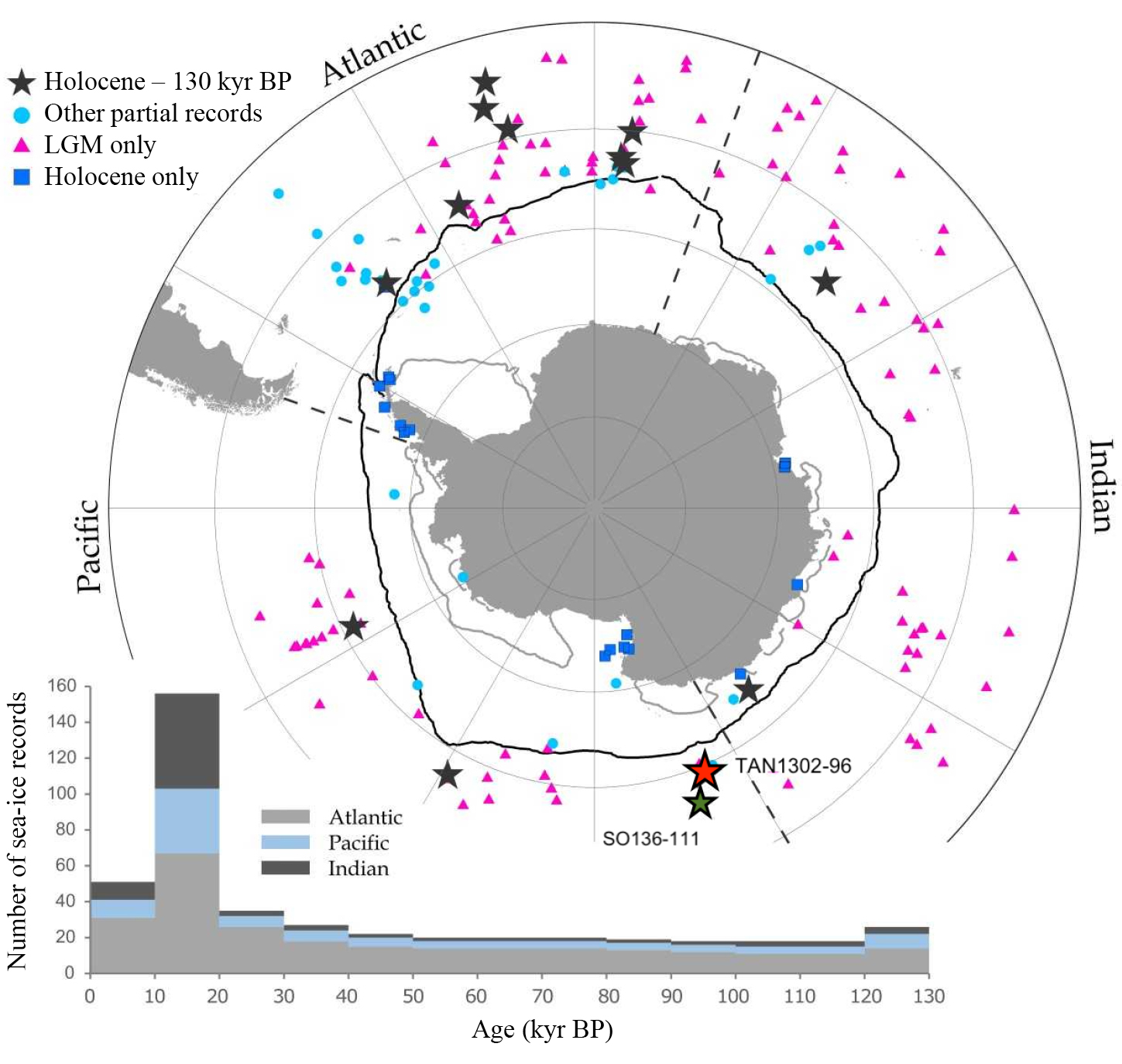
Figure 1: Distribution of marine sea-ice reconstructions. The map shows the locations and temporal resolution of marine sea-ice records, with TAN1302-96 identified as the red star and SO136-111 as the green star. The plot below shows the cumulative number of published records and their temporal scope. Image adapted from Crosta et al. (2022). |
The current glacial–interglacial Antarctic sea-ice dataset is comprised of 14 published marine records that capture the last ~130 kyr (Fig. 1; Chadwick et al. 2022; Crosta et al. 2022). These reconstructions suggest some heterogeneity in spatial and temporal sea-ice coverage, although a general pattern exists across the Southern Ocean. Overall, the winter sea-ice edge quickly retreated during MIS 5e (~130 to 116 kyr BP), and coverage remained relatively low until the mid-glacial, where sea ice appears to have expanded during MIS 4 (beginning around ~65 kyr BP). Sea ice appears to have remained expansive and reached its maximum extent during the LGM (~21 kyr BP) before retreating and remaining relatively low throughout the Holocene.
Case study from the southwestern Pacific
Marine core TAN1302-96, retrieved from the southwestern Pacific sector of the Southern Ocean in 2013 (Fig. 1), is one of the few published marine cores that capture a full glacial–interglacial cycle (Jones et al. 2022). The age model for the core was constructed using a combination of radiocarbon dating and oxygen isotope stratigraphy, which was correlated to a global average of 57 records known as the LR04 benthic stack (Lisiecki and Raymo 2005). Using a diatom-based transfer function known as the Modern Analog Technique (Crosta et al. 1998), past summer sea-surface temperature (SSST) and winter sea-ice concentration (WSIC) were estimated back to 140 kyr BP. The TAN1302-96 reconstruction is the second glacial–interglacial record from the region, the other being SO136-111 (Crosta et al. 2004; Ferry et al. 2015), which together show a relatively coherent sea-ice history in the region over the last glacial–interglacial cycle (Fig. 2).
The timing of sea-ice expansion in the region suggests that it may not have been a key driver of early CO2 sequestration, as was hypothesized by Kohfeld and Chase (2017). However, the expansion of winter sea ice at the TAN1302-96 core site does appear to have occurred at approximately the same time as a vertical displacement of the Antarctic Intermediate Water (AAIW) and Upper Circumpolar Deepwater (UCDW) interface, as inferred from regional benthic carbon isotopes (δ13C) from nearby marine cores (Fig. 2). This δ13C record captures the isotopic composition of the waters overlying the sediments, representing periods when they were bathed primarily by UCDW (low %AAIW) or AAIW (high %AAIW). Changes in the benthic isotopic signature are therefore interpretated as changes in water-mass geometry and regional ocean circulation.
 |
|
Figure 2: (A) WSIC estimates using MAT from SO136-111 (Crosta et al. 2004; Jones et al. 2022); (B) WSIC estimates using MAT from TAN1302-96 (Jones et al. 2022); (C) Antarctic atmospheric CO2 concentrations over 140 kyr BP (Bereiter et al. 2015); (D) δ13C data from nearby cores MD06-2990/SO136-003, MD97-2120, and MD06-2986 (Ronge et al. 2015); (E) %Antarctic Intermediate Water (%AAIW) as calculated in Ronge et al. (2015), which tracks when core MD97-2120 was bathed by AAIW (green) or Upper Circumpolar Deep Water (UCDW) (blue). Note that the %AAIW y-axis is inverted such that low %AAIW is represented in blue and high %AAIW is represented in green. Figure taken from Jones et al. (2022). |
The findings from TAN1302-96 support the hypothesis put forth in Ronge et al. (2015) that the influx of low-density summer melt increased the buoyancy of the AAIW formed in the region, inhibiting its subduction and altering the volume and geometry of both AAIW and UCDW. This process, combined with a reduction in the outgassing of upwelled carbon-rich waters (i.e. the "capping" mechanism), enhanced deep-ocean stratification, and reduced upward mixing of carbon-rich waters, could have led to an increase in the glacial deep-ocean carbon pool. Taken collectively, the expansion of winter sea ice appears to have potentially influenced both the circulation of the ocean and the outgassing of CO2, which may have led to an increase in marine carbon storage.
Future work
In order to substantiate these hypotheses and better understand the role of sea ice in glacial–interglacial CO2 variability, additional records are needed from across the Southern Ocean. Specifically, transects of well-dated cores from each ocean basin would provide both: (1) critical information to constrain the timing and magnitude of sea-ice expansion, and (2) key information on underlying sea-ice and ocean dynamics. The work by the PAGES working group Cycles of Sea Ice Dynamics in the Earth System (C-SIDE; pastglobalchanges.org/c-side) has advanced our collective understanding of past sea-ice coverage by producing a number of new long-duration records and highlighting the gaps in the current knowledge.
affiliations
1School of Resource and Environmental Management, Simon Fraser University, Burnaby, BC, Canada
2Department of Geography, University of California, Los Angeles, USA
3Department of Environmental Sciences, Simon Fraser University, Burnaby, BC, Canada
4School of Earth and Environmental Sciences, University of Queensland, Brisbane, Australia
5Université de Bordeaux, CNRS, Pessac, France
contact
Jacob Jones: jbjones@ucla.edu
references
Bereiter B et al. (2015) Geophys Res Lett 42: 542-549
Chadwick M et al. (2022) Clim Past 18: 1815-1829
Crosta X et al. (1998) Paleoceanography 13: 284-297
Crosta X et al. (2004) Mar Micropaleontol 50: 209-223
Crosta X et al. (2022) Clim Past 18: 1729-1756
Delmas R et al. (1980) Nature 284: 155-157
Ferrari R et al. (2014) Proc Natl Acad Sci USA 111: 8753-8758
Ferry AJ et al. (2015) Paleoceanography 30: 1525-1539
Jones J et al. (2022) Clim Past 18: 465-483
Kohfeld KE, Chase Z (2017) Earth Planet Sci Lett 472: 206-215
Lisiecki LE, Raymo ME (2005) Paleoceanography 20: PA1003
Martin JH (1990) Paleoceanography 5: 1-13
Neftel A et al. (1982) Nature 295: 220-223
Ronge TA et al. (2015) Paleoceanography 30: 23-38
Matthew Chadwick![]()
Past warm periods serve as an analog for the impacts of future warming. Reconstructions of Antarctic sea ice from 130,000 years ago show a reduction in sea-ice extent relative to the present, with the patterns of retreat varying between regions of the Southern Ocean.
Why 130,000 years ago?
Between 130,000 and 116,000 years ago was the time interval known as Marine Isotope Stage (MIS) 5e. Global average temperature during MIS 5e is estimated to have been 2°C warmer than the pre-industrial (Fischer et al. 2018) and similar to what is predicted for 2100 (Meredith et al. 2019). Therefore, investigating the environmental conditions during MIS 5e can provide an analog for the likely environmental and climatic impacts of current and future anthropogenic warming. High latitudes have a greater sensitivity to climatic changes and can amplify the impacts of rising temperatures through feedbacks in the ocean and cryosphere; therefore, studying polar regions is particularly important to understand the climatic impacts of a warming world.
Why Antarctic sea ice?
Antarctic sea ice is a crucial component of the global climate system, due to its high albedo (reflectivity) and the influence it has as a barrier to gas exchange between the atmosphere and ocean (Rysgaard et al. 2011). Sea ice also helps to stabilize Antarctic ice shelves and ice streams by protecting them from wave and ocean swell (Massom et al. 2018) and is a key habitat for many Antarctic organisms (Arrigo 2014).
How is past Antarctic sea ice reconstructed?
As discussed by Armbrecht (p. 78), McClymont et al. (p. 82), and Nixon (p. 84) numerous proxy records can be used to reconstruct past changes in polar sea ice. For the Antarctic, the most robust and well-studied of these proxies are the species assemblage of diatoms, a group of photosynthesizing siliceous microalgae, preserved in marine sediments. Different species of diatoms have different environmental preferences and by studying the species assemblages in seafloor sediments throughout the modern Southern Ocean, a reference database can be built comparing seafloor sediment species assemblages to present environmental conditions (Crosta et al. 1998; Esper and Gersonde 2014). The diatom assemblages preserved in marine sediments from 130,000 years ago can be compared to this reference dataset to reconstruct the past sea-ice concentrations (Chadwick et al. 2022a).
How did winter sea-ice concentrations vary throughout the Southern Ocean during MIS 5e?
The reconstructed patterns and trends in Antarctic winter sea-ice concentrations in Chadwick et al. (2022a) show substantial variation between the three ocean basin sectors (Atlantic, Indian and Pacific) of the Southern Ocean (Fig. 1). The Atlantic-sector sea-ice records (lightest blue shading in Fig. 1) show very low winter sea-ice concentrations in early MIS 5e (~131,000–130,000 years ago), followed by a substantial increase to a maximum around 127,000–126,000 years ago. In contrast to the prominent minimum and maximum in Atlantic-sector sea-ice concentrations, the Pacific-sector records (darkest blue shading in Fig. 1) show very little variability in sea-ice concentrations. All the Pacific-sector records show largely consistent sea-ice concentrations throughout MIS 5e, and the two more southerly cores are the first records where the core site was located beneath winter sea ice throughout MIS 5e. The Indian-sector records (mid-blue shading in Fig. 1) show more variability in sea-ice concentration than in the Pacific sector, but at a higher frequency than the variability in the Atlantic sector. Millennial-scale sea-ice variability in the Indian sector during MIS 5e results in a series of sea-ice concentration maxima and minima, with a greater proportion of high sea-ice periods during earlier MIS 5e followed by a transition to more intervals of low sea ice (Fig. 1) after 125,000 years ago.
 |
|
Figure 1: September sea-ice concentrations for the end of Termination II and early to mid MIS 5e from nine marine sediment cores. Figure modified from Chadwick et al. (2022a). |
How did MIS 5e Antarctic sea-ice extent compare to today?
The sea-ice concentrations reconstructed for MIS 5e (Chadwick et al. 2020; Chadwick et al. 2022a) can be used to estimate where the winter sea-ice edge reached, which can then be compared to its modern position (Fig. 2). During early MIS 5e, the Antarctic winter sea-ice extent reached a minimum of roughly 62% of its modern area, with this increasing slightly, to roughly 71%, by mid MIS 5e. During early MIS 5e, the largest reduction in sea-ice extent, to 58% of its modern extent, was in the Atlantic sector, where the winter sea-ice edge was located roughly 5° latitude south of its modern position (Fig. 2). During mid-MIS 5e, the winter sea-ice edge in the western Atlantic sector expanded by approximately 5–8° latitude, placing it to the north of its modern position (Fig. 2). Chadwick et al. (2022b) hypothesized that this expansion in the western Atlantic sector is a result of the release of large amounts of meltwater and icebergs from the Antarctic ice sheets that outflow into this region of the Southern Ocean. This high outflow of meltwater and icebergs from the Antarctic continent was likely influenced by the sea-ice minimum in early MIS 5e allowing the greater penetration of warmer waters into embayments and under floating ice shelves, promoting their melting and breakup.
Unlike the Atlantic sector, the Indian and Pacific sectors show a greater consistency between early and late MIS 5e, with minimal change in the position of the winter sea-ice edge (Fig. 2). In the Pacific sector, the reduction in MIS 5e winter sea ice relative to today is greatest in the western part of the sector, where it was located roughly 3–4° latitude south of its modern position (Fig. 2). This contrasts to the eastern Pacific sector where the winter sea-ice edge was located < 2° latitude south of its modern position (Fig. 2). In the Indian sector, although the average position of the winter sea-ice edge is largely consistent between early and mid-MIS 5e (Fig. 2), the millennial-scale variability previously discussed means that the position of the winter sea-ice edge will have varied a lot around this average (Fig. 1). Chadwick et al. (2022a) hypothesized that the millennial-scale variability in the Indian-sector winter sea-ice extent is due to the influence of Southern Ocean fronts and surface water masses migrating north and south.
 |
|
Figure 2: September winter sea-ice extent during early and mid-MIS 5e (blue lines) compared to the modern (1981–2010) September sea-ice extent (solid grey line). For the MIS 5e September winter sea-ice extent, the dashed line marks the areas that are less robustly constrained. MIS 5e sea-ice extent is estimated using data from marine sediment cores presented in Chadwick et al. (2020; 2022a). |
What does this mean for the future?
Although the warmer climate during MIS 5e was driven by different forcings than current anthropogenic warming, it still presents an excellent analog for how the climate system is likely to respond to increasing global temperatures. The reconstructions of Antarctic sea ice during MIS 5e indicate that in the future we could see a substantial reduction in Antarctic winter sea-ice extent, to 62% of its modern extent, but that this reduction will not be uniform across the Southern Ocean. The greatest sea-ice losses are expected in the Atlantic sector, with the Pacific-sector sea-ice extent seemingly more resilient to a warming climate. The retreat of Antarctic sea ice in the future has many knock-on consequences for the global climate system, one of which is the likely loss of a substantial volume of the Antarctic Ice Sheet, as evidenced during MIS 5e by the release of meltwater and icebergs into the Atlantic sector (Chadwick et al. 2022a, b).
affiliation
British Antarctic Survey, Cambridge, UK
contact
Matthew Chadwick: m.chadwick@cornwall-insight.com
references
Arrigo KR (2014) Annu Rev Mar Sci 6: 439-467
Chadwick M et al. (2020) Quat Sci Rev 229: 106134
Chadwick M et al. (2022a) Clim Past 18: 129-146
Chadwick M et al. (2022b) Mar Micropaleontol 170: 102066
Crosta X et al. (1998) Paleoceanography 13: 284-297
Esper O, Gersonde R (2014) Palaeogeogr Palaeoclimatol Palaeoecol 399: 260-283
Fischer H et al. (2018) Nat Geosci 11: 474-485
F. Chantel Nixon![]()
Sea ice is an important variable affecting Arctic coastlines, influencing beach morphology and the stranding of whales and driftwood. For ancient beaches, these proxies can provide an archive of Holocene sea-ice dynamics.
The water's edge: Beaches
Sea ice is an essential player in the construction, protection, and erosion of Arctic beaches because it regulates wave climate and heat delivery to the coast, influences nearshore currents, and transports sediment on- and offshore. For example, in summers, when the landfast ice does not melt away, beach formation does not occur (e.g. Funder et al. 2011). A long open-water season, on the other hand, allows waves and currents to modify the shoreline: building beaches or eroding coastal bluffs.
The history of Holocene coastal landscape development has been preserved in many places across the circumpolar Arctic due to glacioisostatic adjustment following deglaciation, causing a fall in relative sea-level (RSL) – the process responsible for the spectacular flights of raised beaches up to hundreds of meters above modern sea level (MSL; Fig. 1). Determining the ages of such raised beaches is most often accomplished via radiocarbon dating organic matter incorporated in or on their surfaces, or, less frequently, using optically stimulated luminescence dating of buried beach sediments (Simkins et al. 2015). Holocene wave climate histories, and, accordingly, summer sea-ice conditions, can be reconstructed by combining well-dated RSL curves with observations of the presence or absence of raised beach ridges, beach-ridge morphology, degree of beach-cobble roundness, and sea-ice-pushed boulders (e.g. Forbes and Taylor 1994; Funder et al. 2011; St-Hilaire-Gravel et al. 2010).
Wood and whales
Sea ice also controls access to the coast for drifting organic matter like wood and whale carcasses, and records of past sea-ice severity in coastal zones may be developed from such data (e.g. Dyke et al. 1997; Dyke et al. 1996; Hole and Macias-Fauria 2017). Interpretation of these proxies, however, is not a straightforward case of less sea ice enabling more driftage. Arctic driftwood, which originates in the vast boreal forests of North America and Eurasia, must spend one to 15 years traversing the Arctic Ocean, drifting with one or both of the two major surface currents (the Beaufort Gyre and the Transpolar Drift) before it has any chance of becoming stranded on a barren Arctic beach or being exported to the North Atlantic (Tremblay et al. 1997). If the driftwood isn't quickly frozen into sea ice at its entry point to the Arctic Ocean and advected off the continental shelves by local currents, it becomes waterlogged and sinks within six to 17 months (the range depends on the species and the part of the tree that is adrift; Häggblom 1982) or gets blown back onshore by storms. After traveling around the Arctic Ocean on multiyear sea ice for several years and once again in proximity to land, access is required for stranding; if the coastal zone is locked up below thick sea ice, driftwood cannot make landfall. The spectacular but vanishing landfast, multiyear sea-ice ice shelves of northern Ellesmere Island, Canada, attest to this phenomenon: 69 radiocarbon-dated samples of driftwood collected from behind the ice shelves (stranded prior to ice-shelf establishment and the onset of coastal blockage) record a clear hiatus in driftwood deposition from around 5500 cal yr BP until breakup of the ice shelves and re-opening of these high Arctic fjord coasts, a process which started in the 1950s (England et al. 2008).
 |
|
Figure 1: (A) Rare "finger delta" (Forbes and Taylor 1994) with prominent, ice-pushed ridges on western side and narrow summer shore lead. Shore lead appears as a black, coast-parallel strip separating white sea ice and grey beaches (Photo credit: National Air Photo Library, Chad's Point, Melville Island, Northwest Territories, Canada; 1950). Numbers indicate elevations of paleoshorelines in meters above MSL. (B) Lithograph showing "log found in M'Clure Strait drifting eastward with ice". From Bernier's 1910 Report on the dominion of Canada government expedition to the Arctic Islands and Hudson Strait on board the D.G.S. Arctic (published by Government Printing Bureau, Ottawa). (C) Driftwood logs stranded on a modern beach on the Kara Sea, Russia (Photo credit: Vadim Simonsen, 2018). (D) Glacioisostatically uplifted raised gravel beach ridges, Varanger Peninsula, Barents Sea, Norway (Photo credit: Chantel Nixon, 2020). (E) Same location as (D) with transgressive erosional scarp shown on the left (Photo credit: Chantel Nixon, 2020). |
If sea ice in the shore zone is highly mobile, winds and currents can transport it onshore, resulting in the formation of sea-ice push ridges (Forbes and Taylor 1994). Sea-ice push can excavate older sediments, including any driftwood they contain, from below MSL and redeposit them alongside modern wood on the same shoreline, especially if RSL is rising. On Eglinton Island in the western Canadian Arctic, for example (where RSL fell to an offshore lowstand in the late Holocene, but is now rising), cut and prepared timber was observed alongside 3000-year-old driftwood (Nixon et al. 2016). As long as it can be demonstrated that the older driftwood has not moved downslope from higher elevations, such assemblages provide not only a minimum age for the onset of RSL rise, but also clear evidence for the consistent development of mobile, multiyear sea ice and summer shore leads over the same period.
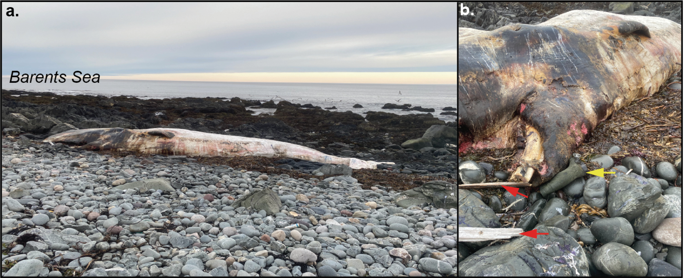
Unlike driftwood, whale bones found on Arctic beaches, most commonly those of the bowhead whale (Balaena mysticetus), require open water for stranding, because when the whales die, their bloated carcasses float for some time before either sinking or being driven ashore by waves and currents (Fig. 2). Once stranded, they decompose, leaving behind only skeletal material, which can be radiocarbon dated. The annual migrations of bowhead whales reflect their preference for floe-edge habitat (Dyke and Morris 1990), although they are wary of becoming trapped beneath multiyear ice. Earlier studies have shown that reduced summer sea-ice conditions in the central Canadian Arctic Archipelago enabled bowhead whales to migrate well beyond their current range several times during the Holocene, with peak abundances between 9500 and 12,800 cal yr BP (Dyke and Morris 1990). Numerous subfossil whale bones have also been documented from Norway, Greenland, Russia, and Antarctica, although many of these reflect historic whaling-era activity (ca. 17th–early 20th centuries) and have not generally been applied in reconstructions of past sea-ice conditions as they have in the Canadian Arctic.
New directions in driftwood research
 |
|
Figure 2: (A) Beached sperm whale (Physeter macrocephalus) on northwestern Varanger Peninsula, northern Norway, some 500–700 km south of the winter floe edge (Photo credit: Chantel Nixon, 2020). (B) Close-up of sperm whale head resting on cobbles and other driftage: a plastic boot (yellow arrow), and driftwood (red arrows; Photo credit: Chantel Nixon, 2020). |
Determining the precise origin of Arctic driftwood provides insight into changes in driftwood trajectories across the Arctic Ocean, which are influenced by changes in the positions of the Beaufort Gyre and Trans-polar Drift (Tremblay et al. 1997). Driftwood provenancing has so far been accomplished with dendrochronology (for recent driftwood; e.g. Linderholm et al. 2021) or by identification of the wood to its genus or species level with the broad and unverified assumption that, of the two most common genera of Arctic driftwood, Larix and Picea, Larix originates from Siberia and Picea from North America (Dyke et al. 1997). New techniques exploring isotopic ratios in driftwood (strontium, for example) are currently being investigated to improve provenancing (Hole et al. 2022).
To reconstruct more robust paleo-sea-ice histories using coastal proxies, the whale-bone, driftwood, and raised-beach data should be examined together where possible (e.g. Dyke and Morris 1990). Nonetheless, the spatially and temporally low-resolution nature of such records means that they are better suited to providing a broad framework for Holocene sea-ice severity into which higher-resolution paleo-sea-ice studies, such as those derived from marine sediment cores, may fit. Future research directions should also focus on filling in geographic gaps along the Russian Arctic coast (Hole and Macias-Fauria 2017) and Antarctica, as well as exploring new potential proxies for past sea-ice conditions in the coastal zone with materials such as pumice from Icelandic volcanic eruptions (Farnsworth et al. 2020).
affiliation
Department of Geography, Norwegian University of Science and Technology, Trondheim, Norway
contact
F. Chantel Nixon: chantel.nixon@ntnu.no
references
Dyke AS et al. (1996) Arctic 49: 235-255
Dyke AS et al. (1997) Arctic 50: 1-16
England JH et al. (2008) Geophys Res Lett 35: L19502
Farnsworth WR et al. (2020) Quat Sci Rev 250: 106654
Forbes DL, Taylor RB (1994) Prog Phys Geogr 18: 59-89
Funder S et al. (2011) Science 333: 747-750
Häggblom A (1982) Geografiska Annaler 64: 81-94
Hole GM, Macias-Fauria M (2017) J Geophys Res Oceans 122: 7612-7629
Hole GM et al. (2022) Palaeogeogr Palaeoclimatol Palaeoecol 590: 110856
Linderholm HW et al. (2021) Polar Sci 29: 100658
Nixon FC et al. (2016) Boreas 45: 494-507
Simkins LM et al. (2015) J Quat Sci 30: 335-348
Erin L. McClymont![]() 1, M.J. Bentley1, D.A. Hodgson1,2, C.L. Spencer-Jones1, T. Wardley1, M.D. West1, I.W. Croudace3, S. Berg4, D.R. Gröcke5, G. Kuhn6, S.S.R. Jamieson1, L.C. Sime2 and R.A. Phillips2
1, M.J. Bentley1, D.A. Hodgson1,2, C.L. Spencer-Jones1, T. Wardley1, M.D. West1, I.W. Croudace3, S. Berg4, D.R. Gröcke5, G. Kuhn6, S.S.R. Jamieson1, L.C. Sime2 and R.A. Phillips2
Where snow petrels forage is predominantly a function of sea ice. They spit stomach oil in defence, and accumulated deposits at nesting sites are providing new opportunities to reconstruct their diet, and, in turn, the sea-ice environment over past millennia.
Antarctic sea ice is important for the climate system, because it influences planetary albedo, ocean–atmosphere heat and gas exchange, and the formation of intermediate and deep water masses which store heat and carbon (Wang et al. 2022). Sea ice also supports unique ecosystems, with the productivity of different species linked to the seasonal and spatial changes in light and nutrient availability (Meredith et al. 2019). Antarctic sea ice is complex, including seasonal and multiyear sea ice of varying albedo and thickness. The sea ice is also broken by open waters which range in scale from small and ephemeral leads (<1 m to ~1 km) to more persistent polynyas (~1000–400,000 km2), which can drive high primary productivity and ocean–atmosphere heat and gas exchange (Arrigo and van Dijken 2003).
The instrumental record has been characterized by regionally variable trends in Antarctic sea-ice extent since the 1970s, but with no overall trend until a decrease began in 2015 (Wang et al. 2022). Understanding what this means for future sea-ice–climate interactions is complicated: the short instrumental records and the challenges of modeling such a complex environment mean we have low confidence projecting sea-ice extent this century (Fox-Kemper et al. 2021).
Paleoclimate archives have extended the instrumental record back through time. Past sea-ice margins and seasonal sea-ice zones have been mapped, largely drawing on fossil diatom assemblages and geochemical markers in marine sediments (Xiao et al. 2016; Crosta et al. 2022). Polynyas have been indicated by changing bottom current flows (Sprenk et al. 2014) or intervals of high biological productivity (Smith et al. 2010). Marine aerosols in ice cores have also revealed regional-scale changes to sea-ice extent and biological productivity (Goto-Azuma et al. 2019).
Relatively little is known about the past properties of the sea ice away from the margins, and even less about the sea-ice ecosystem, beyond those organisms preserved in the microfossil record. However, analyses of stomach-oil deposits generated by snow petrels (Pagodroma nivea) at their nesting sites above the Antarctic Ice Sheet have provided new insights: radiocarbon dating has confirmed that these seabirds were present onshore during the Last Glacial Maximum (~23–19 kyr before present (BP)), even when sea-ice extent was likely doubled relative to today (Thatje et al. 2008). But where were the petrels foraging, and was their diet the same as now? What were the sea-ice conditions where they foraged, and how have these changed over time? These questions are beginning to be answered by exploiting the unique stomach-oil archives to read the climate stories.
 |
|
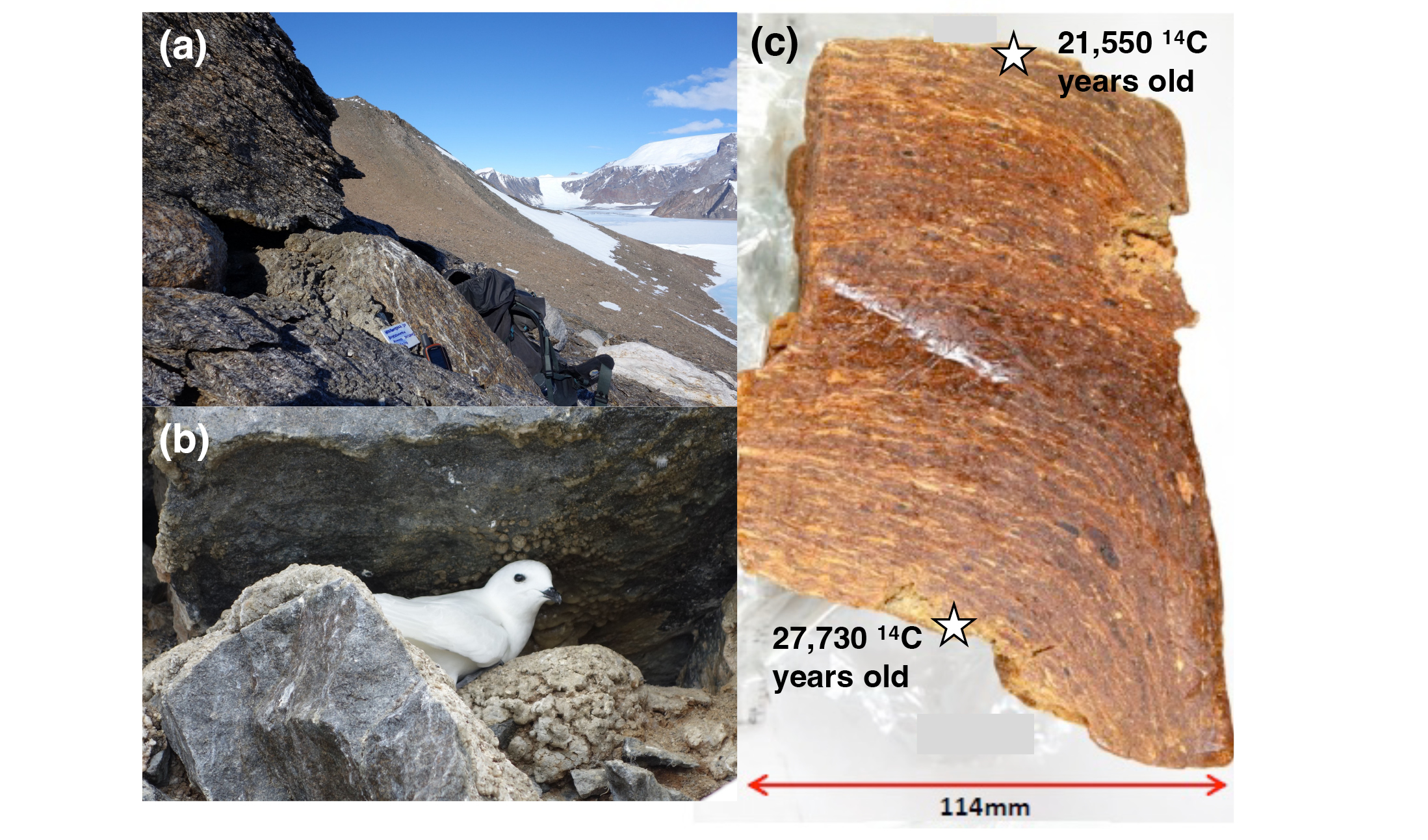
Figure 1: Snow petrels nest in rock crevices above the Antarctic Ice Sheet, which may be several hundred kilometers from the sea (Photo credit: Dominic Hodgson); (B) The defensive regurgitation of stomach oils has led to the accumulation of deposits in front of the snow petrel nest (Photo credit: Dominic Hodgson); (C) Vertical section through stomach-oil deposit WMM7, showing distinct layers building up through time at rates of up to 30 mm per 1000 years |
Snow petrels as sea-ice reporters
Snow petrels are closely associated with Antarctic sea ice, where they are present year-round at the margins and in leads and polynyas (Ainley et al. 1984). During the summer breeding season, they nest in crevices, under boulders, and in scree slopes on the mountains (nunataks) which poke through the Antarctic Ice Sheet (Fig. 1). They continue to forage in the sea ice, traveling hundreds of kilometers from their nests, returning with an energy-rich stomach oil generated from partially digested krill, squid, and fish. The oil is regurgitated as a defense mechanism against predators, and can accumulate around the nest entrance over hundreds or thousands of years (Hiller et al. 1995; Berg et al. 2019; McClymont et al. 2022). The deposits contain a mixture of stomach oils, guano, feathers, and wind-blown sediments (Fig. 1).
The close association of snow petrels with the sea ice means that the deposits are both an archive of snow petrel diet and the sea-ice environment where they fed. For example, several Antarctic seabirds vary the relative contributions of krill and fish in their diet in response to changing prey availability (Fijn et al. 2012). Isolating the biochemical fingerprints of those prey allows us to reconstruct past diets, for example, identifying krill from elevated copper and specific fatty acid distributions (McClymont et al. 2022). Some deposits have also yielded climate proxies more commonly used in marine sediments, including sea-ice diatoms (Berg et al. 2019).
A new archive of sea-ice environments at the onset of the Last Glacial Maximum
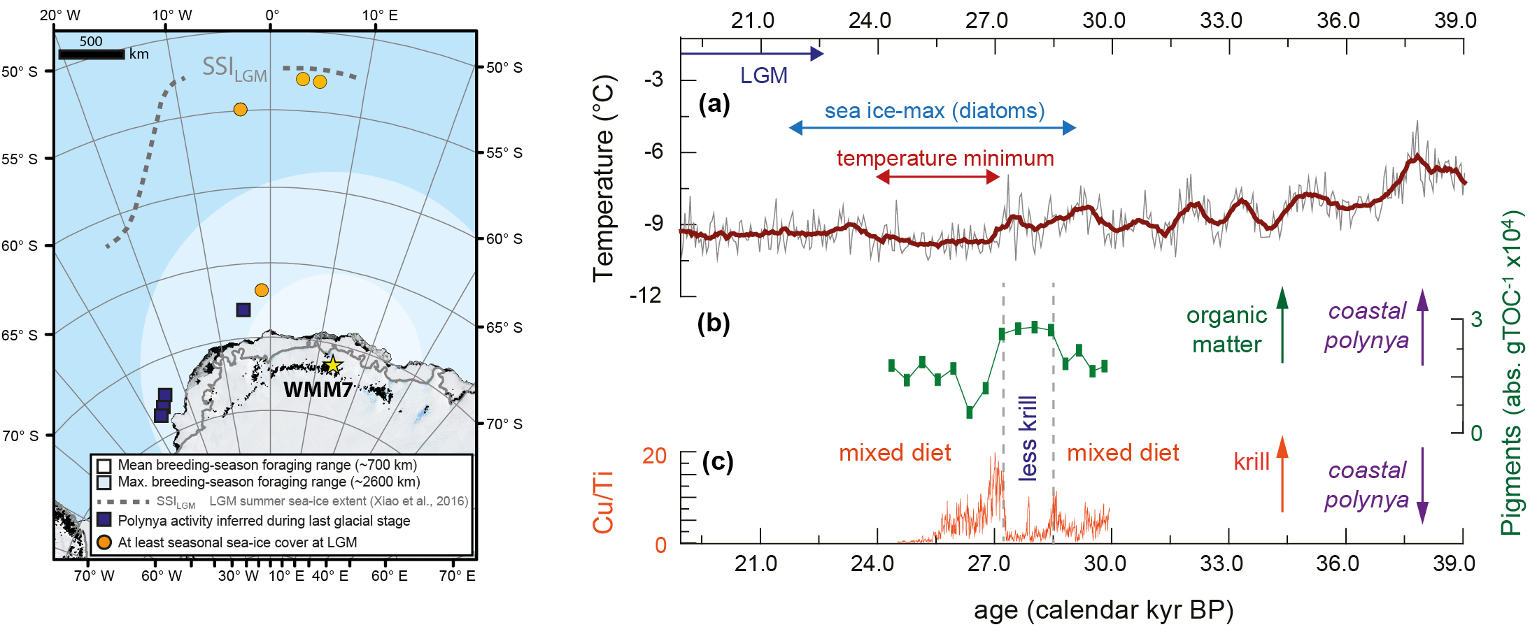
Although the global Last Glacial Maximum occurred ~23–19 kyr BP, maximum Antarctic sea-ice extent was likely reached earlier, ~29–22 kyr BP (Xiao et al. 2016; Goto-Azuma et al. 2019). We analyzed a stomach-oil deposit spanning ~30–24 kyr BP from Untersee, Dronning Maud Land. As snow petrel foraging ranges are limited by the need to return to the nest site, this deposit integrates information about sea-ice environments within ~1000 km of the coastline, in the Atlantic sector of the Southern Ocean (Fig. 2). Stable accumulation rates of the deposit suggest continuous snow petrel nest occupation even as the climate was cooling and sea ice was expanding (McClymont et al. 2022).
 |
|
Figure 2: Left: Dronning Maud Land stomach-oil deposit WMM7 reveals changing sea-ice conditions offshore as summer sea ice expands. Right: (A) Antarctic ice-core δD record of atmospheric temperature, noting cooling ~24-27 cal kyr BP; (B) Photosynthetic pigments and (C) Copper (Cu) inputs to Untersee stomach-oil deposit, WMM7. An interval of relatively reduced Cu plus shifting fatty acid distributions (not shown) and pigments indicates a reduced contribution from krill to the snow petrel diet, interpreted to reflect coastal polynya development. Figures modified from McClymont et al. (2022). |
Using a range of proxy indicators we showed that the snow petrel diet changed through time. Overall, a mixed diet of fish, squid and krill was recorded. However, a ~1000 yr interval when krill was a minor diet component was revealed by a loss of krill fatty acids and copper (Fig. 2). The loss of krill seems likely to reflect a shift in foraging habitat to more coastal waters. But does this mean that the snow petrels were foraging at sea-ice margins which had retreated closer to the coast? This seems unlikely, as this deposit coincides with the maximum sea-ice extent, and the sea-ice margin lay far beyond the snow petrel foraging range (Fig. 2).
To resolve this conundrum, we inferred that the low-krill interval could instead reflect the opening of coastal polynyas, perhaps driven by more intense katabatic winds or a shift in the margins of the Antarctic Ice Sheet (McClymont et al. 2022). This interpretation supports the hypothesis that polynyas were important biological refugia for Antarctic ecosystems during glaciations (Thatje et al. 2008).
Outlook
Snow petrel stomach-oil deposits are revealing new information about how Antarctic seabird diets have changed through the transition to more extensive sea ice during the last glacial stage, and its subsequent retreat through the Holocene. Our results complement and extend those from marine sediments, microfossils, and ice cores, by providing regionally focussed, high-temporal-resolution records of conditions behind the sea-ice margins. By expanding our analyses to a wider network of deposits and biochemical proxies, we hope to generate new, long-term biological records of Antarctic sea ice which can be used to test and explore climate models of past, present, and future.
Acknowledgements
This research has been supported by the European Research Council H2020 (ANTSIE; grant no. 864637), the Leverhulme Trust (Research Leadership Award), and the Deutsche Forschungsgemeinschaft (DFG) priority program SPP 1158 "Antarctic Research with comparative investigations in Arctic ice areas" (BE4764/5-1).
affiliations
1Department of Geography, Durham University, UK
2British Antarctic Survey, Natural Environment Research Council, Cambridge, UK
3Ocean and Earth Science, University of Southampton, National Oceanography Centre, UK
4Institute of Geology and Mineralogy, University of Cologne, Germany
5Department of Earth Science, Durham University, UK
6Alfred Wegener Institute, Helmholtz-Center for Polar and Marine Research, Bremerhaven, Germany
contact
Erin McClymont: erin.mcclymont@durham.ac.uk
references
Ainley DG et al. (1984) Ornithol Monogr 32. American Ornithological Society, 97 pp
Arrigo KR, van Dijken GL (2003) J Geophys Res: Oceans 108: 3271
Berg S et al. (2019) Geochem Geophys Geosyst 20: 260-276
Crosta X et al. (2022) Clim Past 18: 1729–1756
Fijn RC et al. (2012) Mar Ornithol 40: 81-87
Goto-Azuma K et al. (2019) Nat Commun 10: 3247
Hiller A et al. (1995) Radiocarbon 37: 171-180
McClymont EL et al. (2022) Clim Past 18: 381-403
Smith JA et al. (2010) Earth Planet Sci Lett 296: 287-298
Sprenk D et al. (2014) Clim Past 10: 1239-1251
Thatje S et al. (2008) Ecology 89: 682-692

Getting to the core of sea-ice reconstructions: Tracing Arctic sea ice using sedimentary ancient DNA
Sara Harðardóttir![]() 1,2, J.R. Evans
1,2, J.R. Evans![]() 3, D.M. Grant
3, D.M. Grant![]() 4 and J.L. Ray
4 and J.L. Ray![]() 4
4
A significant gap exists in our understanding of sea-ice variability on geological timescales. Recent advances using sedaDNA captures a larger fraction of the marine biodiversity than classical approaches. Accompanied by developments of new quantifiable sedaDNA-based proxies, a new era in paleo reconstructions may be on the horizon.
In a changing world with accelerating temperature rise, Arctic sea ice is declining at an unprecedented pace. Understanding past conditions of the Arctic cryosphere is key to building future climate projections, which are essential for decision-making and resolutions, e.g. towards our common UN Sustainable Development Goals (Fig. 1). For several decades, the Earth-science community has been looking for proxies (indicators) that can improve reconstructions of past sea-ice changes. Most proxies for past sea ice are records from marine sediments, alongside ice cores and other indicators, such as driftwood and whale macrofossils (reviewed in de Vernal et al. 2013). The most widely used proxies are archives of single-celled marine eukaryotes, termed protists. Several protists preserve well in the sediments owing to their silica frustules (e.g. diatoms), calcium carbonate tests (e.g. foraminifera), or refractory organic compounds (e.g. dinoflagellate cysts). Protist-derived biogeochemical tracers, including highly-branched isoprenoid (HBI) biomarkers, such as sea-ice biomarker IP25 (Kolling et al. 2020) and alkenones (Wang et al. 2021), are also widely used for paleo sea-ice reconstructions. All established sea-ice proxies have considerable limitations, preservation biases, and low taxonomic resolution or coverage, highlighting the need to identify new proxies to corroborate current paleo reconstructions.
In recent decades, sedimentary ancient DNA (sedaDNA) has become a promising new tool for paleo reconstructions. The universal presence of DNA in all cellular organisms and some virus genomes makes it an ideal target molecule. In this article, we describe the latest developments in the application of sedaDNA in paleo sea-ice research, discuss the major challenges in the field, and suggest avenues for advancements.
Current advances in sedaDNA applications for sea-ice reconstructions
The unique diversity of Arctic sea-ice microbiota relative to the water column or seafloor sediments provides distinct targets for sedaDNA queries. sedaDNA application for sea-ice reconstructions does not demand prior knowledge about the site- or time-relevant paleobiodiversity. Analyses can be "tuned" for selective enrichment of functional groups, such as diatoms (Zimmermann et al. 2021), pan-Arctic microbial eukaryotes (Poulin et al. 2011), foraminifera (Pawłowska et al. 2020), taxa associated with sea-ice melting events (Boetius et al. 2013), sea-ice brine-associated viruses (Zhong et al. 2020), prey organisms and parasites of foraminifera (Greco et al. 2021), protist sources of sea-ice biomarkers (Brown et al. 2020), and sea-ice-dependent mammals (Kovacs et al. 2011) (Fig. 1).
sedaDNA measurements uniquely allow us to capture a broad spectrum of organisms in a single sample. Investigations embrace several sequencing technologies that can be used for diverse types of assessments, such as qualitative descriptions of Arctic sea-ice communities (De Schepper et al. 2019; Zimmermann et al. 2021) and quantitative measurements of sea-ice indicator taxa (De Schepper et al. 2019). Many sequencing applications depend on polymerase chain reaction (PCR) technology, which can introduce biases during amplification and significantly impact interpretations. The most advanced approach that both quantifies targeted marine sedaDNA sources and overcomes some PCR biases is metagenomics, using direct shotgun sequencing of the DNA extract. Shotgun sequencing combined with hybridization capture baits for research defined taxa have recently been applied to Southern-Hemisphere sediment records, providing new information about the diversity and authenticity of marine protist DNA signatures up to one million years old (Armbrecht et al. 2022). These advances highlight an exciting and important new avenue of sedaDNA research that can complement classical multi-proxy Arctic sea-ice reconstructions dating back to the Last Interglacial and beyond.
 |
|
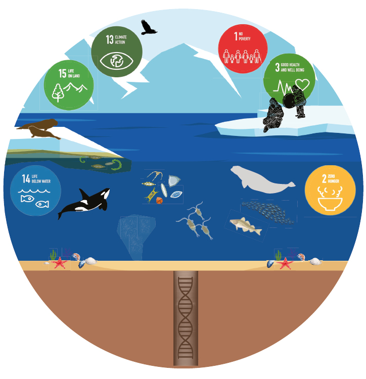
Figure 1: Simplified sketch of Arctic biodiversity, sea ice to the seafloor, illustrating organisms that may leave traces of DNA in the below sediment. As detailed in the United Nations Sustainable Development Goals (SDGs), sea ice can have a large impact on human societies, especially local communities that directly rely on sea ice and the biodiversity related to it. Sea ice is a source of food and income, for example, relevant for SDGs (1) no poverty, (2) zero hunger and, (3) good health and wellbeing. Recognized by the Intergovernmental Panel on Climate Change, the ongoing change in the cryosphere is a global concern; SDG 13 calls for climate actions to sustain the quality of life below water (SDG 14) and life on land (SDG 15). The authors of this article support the SDGs. |
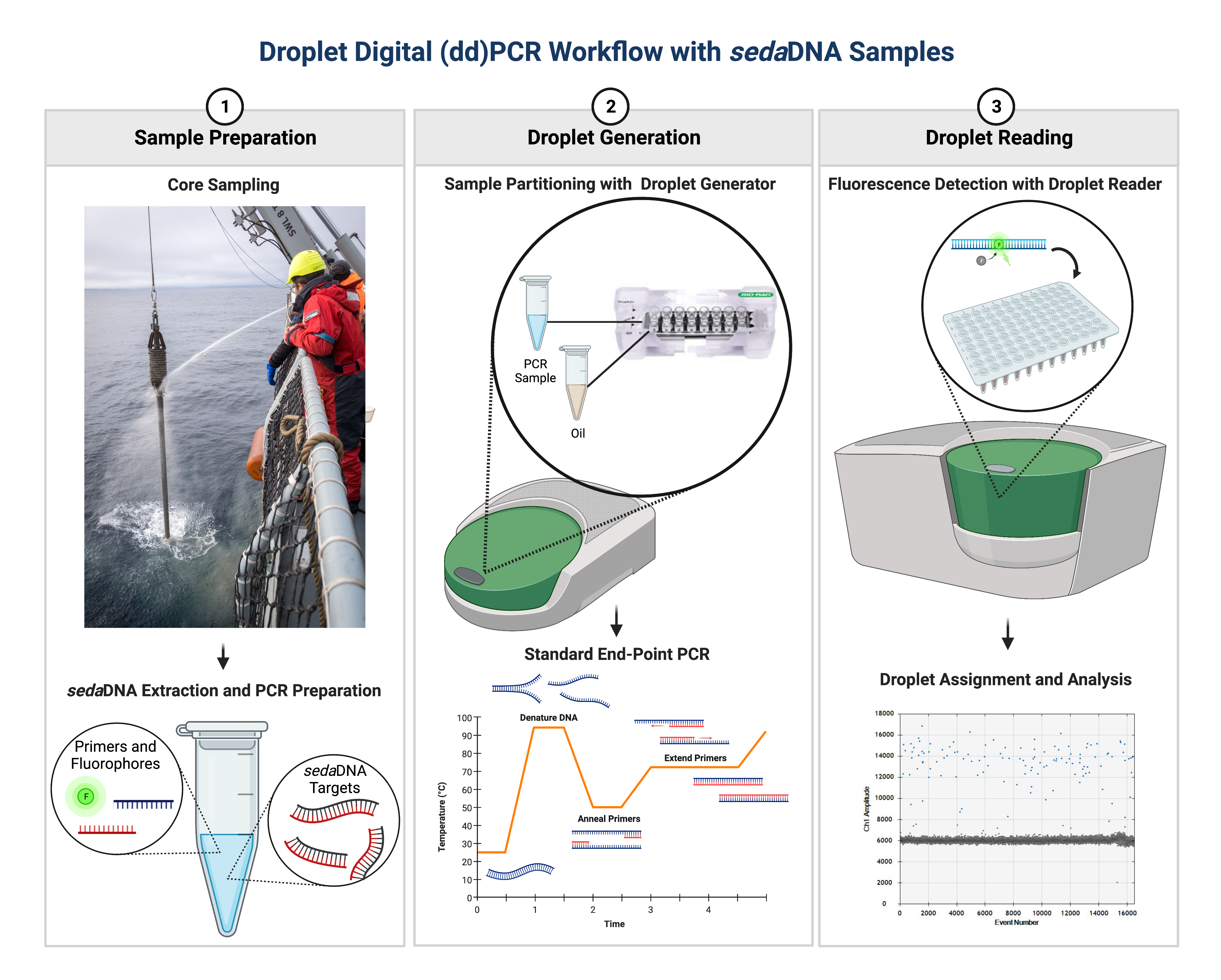
The molecular technologies used in sedaDNA studies are constantly evolving, allowing for developments of quantitative sedaDNA proxies. Specifically, a recent development has been the incorporation of Droplet Digital PCR (ddPCR), which was successfully implemented to quantify the low-abundance of highly informative sea-ice taxa (De Schepper et al. 2019). ddPCR is a powerful tool because it allows the absolute quantification of DNA targets from complex environmental samples. In contrast to the traditional method of real-time quantitative PCR, the ddPCR platform uses end-point quantification of target DNA, which makes it less susceptible to poor amplification efficiencies and PCR-inhibiting molecules commonly found in sedaDNA samples (Hindson et al. 2011; Kokkoris et al. 2021). The immense number of generated droplets delivers highly reproducible measurements and an excellent range in sensitivity that increases the potential to detect lowly abundant taxa (Hindson et al. 2011).
Challenges
The rapidly evolving field of paleogenomics was initially applied to study human evolution, and there is still much to be learned to accomplish optimal applications for past Arctic sea-ice reconstructions. The mineralogical composition of sediments plays a major role in DNA preservation, and we have a limited understanding of DNA-sediment interactions, leading to significantly variable DNA yields across sediment types (Sand and Jelavić 2018); we suspect that the conditions in the Arctic might be favorable. The differences in the preservation of extracellular vs. intracellular DNA and DNA degradation rates in sediments are poorly known. The conditions at the water–sediment interface and bioturbation may also affect the long-term preservation of DNA. Ancient DNA sequences are short, averaging around 100 base pairs (Armbrecht et al. 2021), and most often damaged, which hinders amplification if primers cannot bind to the targets. Available sedaDNA extraction techniques have only moderately been compared. Consequently, the obtained results are difficult to relate and compare, causing a bias as the DNA acquired may not accurately reflect past biodiversity. Temporal constraints have yet to be established, determining how far back in time the method can be applied.
 |
|
Figure 2: Essentials of the general ddPCR workflow for use with sedaDNA applications (created with BioRender.com). Following the acquisition of sedaDNA samples, 20-µL PCR samples (containing a fluorescent DNA reporting dye and sedaDNA template) are partitioned into 20,000 droplets and then PCR-amplified to the end-point. The PCR-amplified droplets in each sample are then analyzed individually for fluorescence intensity, with each droplet classified as positive or negative. Poisson statistics are then applied to the proportion of positive droplets to calculate the absolute number of target DNA molecules in a sample. |
Specifically challenging for sedaDNA application for sea-ice reconstructions is that data from modern conditions such as changes in community structure, and spatial distribution of environmental proxies are rare (e.g. Limoges et al. 2018). The taphonomy of DNA derived from sea-ice-associated organisms, vertical export from sea ice to the seafloor, and its eventual incorporation into marine sediment records are poorly understood. There is also uncertain ontology, as the surface of the DNA can differ between sea ice, the water column, or sediment. Although progress has been made, protists are still largely unrepresented in DNA databases. Many, if not the majority, of the "true" sea-ice-specific species (sea-ice algae), lack DNA and/or morphological references. This occurs for several reasons: sea-ice algae are difficult to collect, culture, and maintain; scientific investigations are limited and often conducted with a high taxonomic resolution; and there are likely still many species unknown to science.
Call for activities
(1) Support taxonomists: The importance of skilled taxonomists in keeping reference databases up to date, and thus making the accurate identification of sea-ice organism genetic signatures in sedaDNA possible, cannot be overstated. "Blue sky" investments must be prioritized for maintaining and cultivating this invaluable expertise. Curated contributions to reference barcode, e.g. Protist Ribosomal Reference database PR2 (Guillou et al. 2012) and metaPR2 (Vaulot et al. 2022), metagenome, plastid, and mitogenome databases with rich associated metadata are essential for the identification of sympagic and sea-ice-associated genetic signatures in sedaDNA.
(2) Build the archive: Bioinformatic advances using supervised machine learning (SML) can be applied to sedaDNA records to extract the sea-ice "needle" from the sedaDNA "haystack". Such data-driven scientific advances are empowered by coordinated research efforts to fill environmental-DNA (eDNA) archives with data from present-day sea ice, the water column, and surface sediments, which reflect different types, thicknesses, and ages of sea-ice cover. eDNA analyses generate community profiles similar to dinoflagellate cyst and diatom assemblages that are used to generate transfer functions. Transfer functions for sea-ice reconstruction based on eDNA community profiling is a tempting possibility. A rich and diverse sea-ice eDNA archive would facilitate rigorous validation to avoid statistical pitfalls. Transfer functions and/or SML algorithms trained on modern eDNA observations, in combination with remote satellite observations and traditional geochemical sea-ice proxies, could then be applied to multi-proxy paleorecords that include sedaDNA to conduct qualitative and, ideally, quantitative extrapolation of past sea-ice extent in the Arctic. It is uncertain to which extent sedaDNA analysis can be applied to historical sediment samples, i.e. non-archive samples that have been collected during the last decades and have been stored either freeze-dried or at 4°C, but their inclusion would certainly make a low-cost contribution toward archive development.
(3) Collaboration and recruitment: The development of sedaDNA into a tool that is informative for sea-ice reconstructions in the Arctic will depend upon continued collaboration between geologists, paleoceanographers, paleoclimatologists, paleoecologists, taxonomists, and molecular ecologists. Shared research cruises, dedicated sessions at international conferences, theoretical and practical training courses, hackathons, international sea-ice sedaDNA collaborative research projects, and cross-disciplinary recruitment programs can help to ensure sample acquisition, strengthen data analysis, encourage competence exchange, and develop training programs for the next generation of Arctic sea-ice researchers.
affiliations
1Glaciology and Climate Department, Geological Survey of Denmark and Greenland, Copenhagen, Denmark
2Département de Biologie, Université Laval, Québec City, QC, Canada
3Department of Earth Sciences, University of New Brunswick, Fredericton, Canada
4NORCE Norwegian Research Centre AS, Climate & Environment Department, Bergen, Norway
contact
Sara Harðardóttir: saha@geus.dk
references
Armbrecht L et al. (2021) ISME Commun 1: 66
Armbrecht L et al. (2022) Nat Commun 13: 5787
Boetius A et al. (2013) Science 339: 1430-1432
Brown TA et al. (2020) Org Geochem 141: 103977
De Schepper S et al. (2019) ISME J 13: 2566-2577
de Vernal A et al. (2013) Quat Sci Rev 79: 122-134
Greco M et al. (2021) J Plankton Res 43: 113-125
Guillou L et al. (2012) Nucleic Acids Res 41: D597-D604
Hindson BJ et al. (2011) Anal Chem 83: 8604-8610
Kokkoris V et al. (2021) Appl Microbiol 1: 74-88
Kolling HM et al. (2020) Geochem Geophys Geosyst 21: e2019GC008629
Kovacs KM et al. (2011) Mar Biodiv 41: 181-194
Limoges A et al. (2018) J Geophys Res Biogeosci 123: 760-786
Pawłowska J et al. (2020) Sci Rep 10: 15102
Poulin M et al. (2011) Mar Biodiv 41: 13-28
Sand KK, Jelavić S (2018) Front Microbiol 9: 2217
Vaulot D et al. (2022) Mol Ecol Resour 22: 3188-3201
Wang KJ et al. (2021) Nat Commun 12: 15
Zhong Z-P et al. (2020) mSystems 5: e00246-20
Zimmermann HH et al. (2021) Paleoceanogr Paleoclimatol 36: e2020PA004091
Letizia Tedesco![]() 1 and Eric Post2
1 and Eric Post2
Sea ice – a unique and extraordinary biome in its nature and dynamics – is under threat. Ocean warming, sea-ice decline, and altered seasonality endanger the simple, vulnerable, and low resilient sea-ice and ice-associated food webs in both polar oceans.
Sea ice is one of the largest biomes on our planet, covering an area up to 14 million km2 in the Arctic Ocean in March 2022 and up to 17 million km2 in the Southern Ocean last September. While Arctic and Antarctic sea ice are similar in many facets, fundamental differences also affect the type of sea-ice biome they are associated with. The fact that the Arctic Ocean is surrounded by land makes the sea ice there more stationary, permanent, and deformed, and with more melt ponds due to a thinner snowpack (Fig. 1a). In contrast, the Southern Ocean surrounds an entire continent. It is affected by abundant precipitation with more snow-ice formation, more mobile sea ice prone to openings, and more young ice formation (Fig. 2a).
Since satellite records began providing reliable observations over 40 years ago, Arctic sea ice has steadily decreased annually in every season, reaching an annual minimum extent in summer, and first-year ice has replaced multiyear ice as the dominant ice type (Stroeve and Notz 2018). During the same period, Antarctic sea ice has shown strong regional and seasonal patterns of variability, with gradual increases in extent until a reversal of this trend in 2016. Since then, it has declined at a rate far exceeding that of Arctic sea ice (Parkinson 2019). Under a warming scenario of at least 2.0°C, the Arctic Ocean is expected to become ice-free throughout September regularly (Notz and Stroeve 2018). Sea ice in the Southern Ocean is also projected to decrease significantly in all seasons during this century in response to warming, with a larger spread of uncertainty in model estimates (Holmes et al. 2022).
The sea ice and ice-associated food webs
Sea ice is an extraordinary multiphase medium comprising a solid ice matrix, liquid salty brines, gas bubbles, and impurities. It is in the brines that a unique ecosystem develops. From viruses, fungi, bacteria, and microalgae to different forms of meio- and macrofauna, an entire food web inhabits sea ice (Figs. 1b, 2b). Compared to the Arctic, Antarctic sea ice is typically more snow-covered, insulated, and permeable, and contains more extensive brines, facilitating access by larger organisms. The most abundant group of organisms found in sea ice is usually tiny algae, which, together with their pelagic counterpart, phytoplankton, form the base of the entire polar marine food web.
In both hemispheres, and in both land-fast and pack ice alike, different algal species, often representing a single functional group, dominate; these include autotrophic flagellates in surface layers, mixed communities in the interior layers, and pennate diatoms in bottom layers (van Leeuwe et al. 2018; Figs. 1b, 2b). Among pennate diatoms, those of the genus Nitzschia are often dominant in both Arctic and Antarctic sea ice. Rotifers and nematodes are more commonly found in Arctic sea ice, while copepods are more commonly found in Antarctic sea ice (Bluhm et al. 2017; Figs. 1b, 2b). Crustaceans dominate under-ice communities. Copepods and amphipods are found in both under-ice environments; dominant taxa include euphausiids in the Southern Ocean and amphipods in the Arctic Ocean (Figs. 1b, 2b). Ice algae support key under-ice foraging species, i.e. Arctic cod (Boreogadus saida) in the Arctic Ocean (Fig. 1a, c) and Antarctic krill (Euphausia superba) in the Southern Ocean (Fig. 2). These species are dependent on the existence of stable sea ice and are key for transferring carbon from primary producers to higher trophic levels, from fish to marine mammals to humans (Figs. 1, 2).
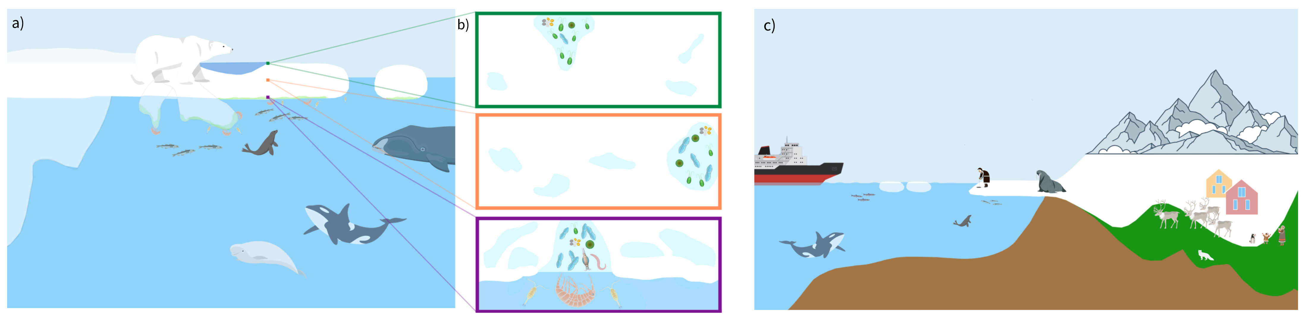 |
|
Figure 1: Schematic representation of the (A) Arctic ice types and ice-associated food web (partly adapted from Bluhm et al. 2017); (B) Arctic sea-ice food web in surface, interior, and bottom layers; and (C) Arctic terrestrial-marine ecological linkages (adapted from Meredith et al. 2022). See Figure 2 for legend keys. |
Sea ice and terrestrial ecology
Strong linkages exist between Arctic marine and terrestrial ecology (Fig. 1c). Sea ice can act as an important ecological corridor, connecting land masses in the Arctic and thereby facilitating the exchange of individuals of some terrestrial species among populations. Moreover, sea ice is an important foraging and predator-escape platform for many species of marine pinnipeds, such as seals and walrus. As sea-ice extent diminishes and ice edges recede from shallow coastal waters, foraging conditions for species such as walrus shift from benthic (i.e. shallow water) to pelagic (i.e. deeper water), increasing foraging time and forcing animals ashore where crowding, trampling and disease transmission can increase (Post et al. 2013; Fig. 1c).
Recent studies have shown that sea-ice variations can modify the proximal abiotic environment on land adjacent to the ocean, influencing tundra vegetation productivity, phenology, and community composition; in some cases, these dynamics can alter the abundance of large herbivores such as caribou (Fauchald et al. 2017; Fig. 1c). Moreover, sea-ice dynamics can alter local abiotic conditions far inland, sometimes resulting in rain-on-snow events that encase reindeer pastures in ice, leading to massive reindeer die-offs (Forbes et al. 2016). The associations between tundra vegetation and Arctic sea-ice decline are complex and difficult to generalize, in some regions reducing shrub growth through local moisture limitation and in other regions promoting shrub growth through local warming and precipitation (Buchwal et al. 2020).
The threat of global warming on polar marine food webs
Ocean warming, sea-ice decline, and altered seasonality are major concerns for polar marine food webs (Figs. 1, 2), which are relatively simple and have low resilience, making them particularly vulnerable to perturbations at all trophic levels. The ongoing environmental changes exert a large stress at the base of the food web, with alterations in abundance, distribution, composition, and seasonality of the microbiota, which may result in major cascading effects.
Lannuzel et al. (2020) produced non-quantitative future expectations of how the changing sea-ice environment will likely impact the sea-ice biogeochemical dynamics and associated ecosystems in the Arctic Ocean. In the short term, sea-ice primary production is projected to generally increase due to the increased light availability after sea-ice and snow thinning, as long as nutrients are plentiful (Tedesco et al. 2019). However, as a consequence of earlier melt onset, the earlier timing of algal blooms is likely to have negative downstream effects on ice-dependent consumers such as copepods, amphipods, and Arctic cod, all of which are dependent on the availability of ice-algal food sources for their overwintering survival (Søreide et al. 2010). Consequently, a decline in conditions of those species feeding preferably on Arctic cod, such as ringed seals, belugas, and bowhead whales (Harwood et al. 2015; Fig. 1a), and the expansion northwards of sub-Arctic species such as capelins and killer whales, are expected (Fig. 1c).
The main population of Antarctic krill inhabiting the Southern Ocean has been found to have contracted significantly southward in response to rapid environmental changes (Atkinson et al. 2019). The changes in the distribution of krill populations directly impact fish, penguins, seals and whales dependent on krill for their survival, and indirectly impact the higher trophic level predators in the food web (Fig. 2a). A similar effort to that of Lannuzel et al. (2020), but focusing on the near-future changes of the Antarctic sea-ice ecosystem, is currently ongoing (Klaus Meiners, personal communication).
Hence, various consequences are to be expected for several ecosystem services. In a rigorous synthesis of the ecosystem services linked to the sea-ice ecosystem, Steiner et al. (2021) highlight that the sea-ice ecosystem supports all four ecosystem service categories: "supporting services" provided in the form of habitat, including feeding grounds and nurseries; "provisioning services" through harvesting, and medicinal and genetic resources; "cultural services" through Indigenous and local knowledge systems, cultural identity, and spirituality, and via cultural activities, tourism and research; and "regulating services" such as climate, through light regulation, the production of biogenic aerosols, halogen oxidation and the release/uptake of greenhouse gasses such as carbon dioxide.
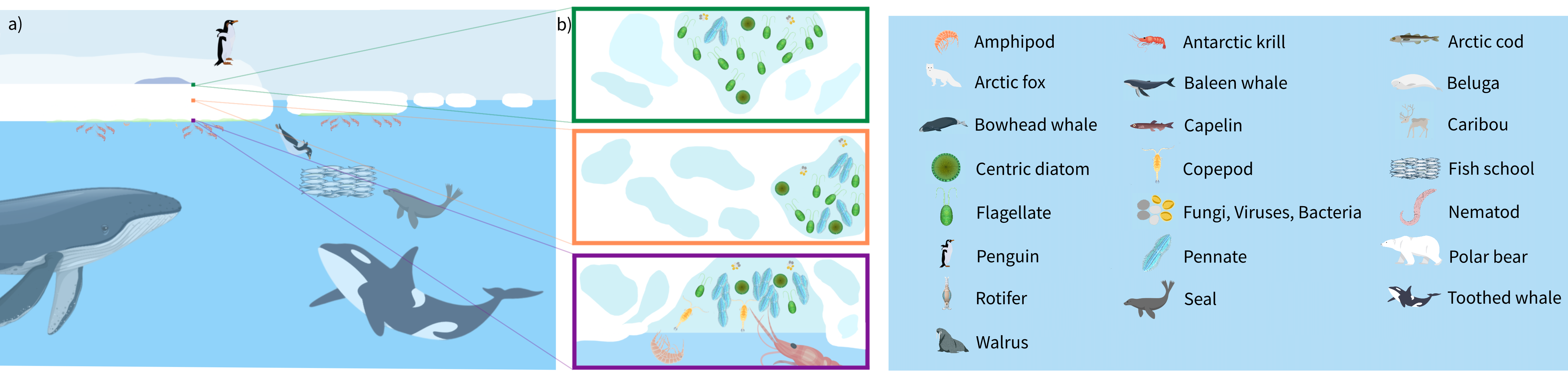 |
|
Figure 2: Schematic representation of the (A) Antarctic ice types and ice-associated food web (partly adapted from Bluhm et al. 2017); and (B) Antarctic sea-ice food web in surface, interior, and bottom layers. |
Steiner et al. (2021) also emphasize that sea-ice ecosystems meet the criteria for ecologically or biologically significant marine areas and deserve specific attention in evaluating marine-protected area planning since conservation could help protect some species and functions. However, the paucity of sea-ice observations hinders our ability to understand, prepare for, and manage the changes. Due to their remote location and common extreme weather conditions, observations in the polar oceans are spatially and temporally sparse, satellite remote sensors have limited applicability, and the quality of sedimentary biological proxies is frequently disturbed.
Our inability to quantitatively predict the ecological changes associated with Arctic sea-ice decline during times of striking changes has led this research topic to be qualified as a "crisis discipline" in "conservation biology" (Macias-Fauria and Post 2018). Given the recent accelerating sea-ice changes in the Southern Ocean and the potential detrimental impacts on the associated ecosystems, we suggest that the ecological consequences of sea-ice changes should be qualified as a "crisis discipline" also in the Antarctic. Urgent knowledge and prompt decisions are needed in polar oceans facing significant uncertainties.
Acknowledgements
LT received funding from the European Union's Horizon 2020 research and innovation programme under grant agreement No 101003826 via project CRiceS (Climate Relevant interactions and feedbacks: the key role of sea ice and Snow in the polar and global climate system) and from the Academy of Finland under grant agreement 335692 via project IMICROBE (Iron limitation on primary productivity in the Marginal Ice Zone of the Southern Ocean – unravelling the role of bacteria as mediators in the iron cycle).
Affiliations
1Marine Research Centre, Finnish Environment Institute, Helsinki, Finland
2Department of Wildlife, Fish, and Conservation Biology, University of California Davis, USA
Contact
Letizia Tedesco: letizia.tedesco@environment.fi
References
Atkinson A et al. (2019) Nat Clim Chang 9: 142–147
Bluhm BA et al. (2017) In: Thomas DN (Ed) Sea ice. John Wiley & Sons Ltd, 394-414
Buchwal A et al. (2020) Proc Natl Acad Sci USA 117: 33,334-33,344
Fauchald P et al. (2017) Sci Adv 3: e1601365
Forbes BC et al. (2016) Biol Lett 12: 20160466
Harwood LA et al. (2015) Prog Oceanogr 136: 263-273
Holmes CR et al. (2022) Geophys Res Lett 49: e2021GL097413
Lannuzel D et al. (2020) Nat Clim Chang 10: 983-992
Macias-Fauria M, Post E (2018) Biol Lett 14: 20170702
Notz D, Stroeve J (2018) Curr Clim Change Rep 4: 407-416
Parkinson CL (2019) Proc Natl Acad Sci USA 116: 14,414-14,423
Post E et al. (2013) Science 341: 519-524
Søreide JE et al. (2010) Glob Change Biol 16: 3154-3163
Steiner NS et al. (2021) Elem Sci Anth 9: 00007
Stroeve J, Notz D (2018) Environ Res Lett 13: 103001
Tedesco L et al. (2019) Sci Adv 5: eaav4830
van Leeuwe MA et al. (2018) Elem Sci Anth 6: 4
CORRIGENDUM
The second part of the paragraph on "The threat of global warming on polar marine food webs” is corrected and modified as follows:
"However, as a consequence of earlier melt onset, the earlier timing of algal blooms is likely to have negative downstream effects on copepods and amphipods, both dependent on the availability of ice-algal food sources for their overwintering survival (Søreide et al. 2010), with repercussions on their consumers, Arctic cods and bowhead whales (Fig. 1a). Consequently, a decline in conditions of ringed seals and belugas (Harwood et al. 2015) feeding mainly on Arctic cod, and the expansion northwards of sub-Arctic species such as capelins and killer whales, are expected (Fig. 1c)."
Ryan L. Fogt![]() 1, Q. Dalaiden
1, Q. Dalaiden![]() 2,3 and M.S. Zarembka1
2,3 and M.S. Zarembka1
Antarctic sea-ice-extent reconstructions provide needed historical context to the large variability depicted in the short satellite observations. However, it is important to be mindful of their uncertainties, especially when comparing reconstructions based on paleoclimatological and instrumental data.
The South Pacific sector of the Antarctic coastline, consisting of the (moving east from the dateline) Ross, Amundsen, and Bellingshausen seas, has demonstrated some of the strongest trends in Antarctic sea-ice extent since the satellite era (1979; Parkinson 2019). The annual mean sea-ice concentration trends (expressed as % per decade) from 1979–2020 (Fig. 1a) show statistically significant increases in the western Ross Sea and decreases in the Bellingshausen Sea near the Antarctic Peninsula. Even with significant trends, these regions are marked with strong interannual sea-ice variability partly influenced by teleconnections from the tropics (Holland and Kwok 2012; Meehl et al. 2016; Purich et al. 2016).
To help place the trends depicted by the short time period of satellite observations in a longer historical context, several sea-ice reconstructions for the South Pacific sector based on both paleoclimatological records and instrumental observations have been created. Abram et al. (2010) used the chemical information from an ice core from the Antarctic Peninsula to reconstruct the annual sea-ice edge in the Bellingshausen Sea (70°W–110°W) in the years 1900–2004. Similarly, a later study by Thomas and Abram (2016) reconstructed the annual mean sea-ice edge at 146°W for the years 1702–2010, marked as a green dot in Figure 1a.
To understand processes behind the sea-ice-extent changes on longer timescales, Dalaiden et al. (2021) combined ice-core and tree-ring-width records with an Earth system model through a data assimilation method to provide annual historical estimates of not only sea-ice extent and concentration, but also the atmospheric circulation (temperature, pressure, winds) during the years 1800–2000. More recently, Fogt et al. (2022) reconstructed seasonal sea-ice extent in the sectors from Raphael and Hobbs (2014) from 1905–2020 using a principal component regression technique that employed observations of pressure and temperature across the Southern Hemisphere, and indices from leading modes of climate variability known to influence Antarctic sea-ice extent. Despite the potential to increase the understanding of historical sea-ice variations from these reconstructions, Fogt et al. (2022) noted a very weak interannual correlation between these datasets, making it challenging to know the reliability and usefulness of each dataset; yet understanding these uncertainties and differences is fundamental to ensure a correct application of the reconstructions.
South Pacific Antarctic sea-ice extent since 1900
Figure 1b shows the annual mean (approximately related to the August–October values for the Abram et al. (2010) reconstruction) sea-ice reconstructions for the Amundsen–Bellingshausen seas (top panel) and Ross–Amundsen seas, along with satellite observations. Importantly, the Fogt et al. (2022) reconstruction was explicitly calibrated to the satellite observations, so it is not surprising that it agrees the best with the observed values in both regions. In contrast, the Dalaiden et al. (2021) reconstructions are not calibrated to observations, but rather are extracted (here, using the Raphael and Hobbs (2014) sectors) from the climate model simulation that is guided by paleoclimatological data. These differences in methodology certainly contribute to the differences among the various reconstructions, since there is more agreement between the paleo-based reconstructions (all except Fogt et al. 2022) than between the paleo-based and instrument-based (only Fogt et al. 2022) reconstructions.
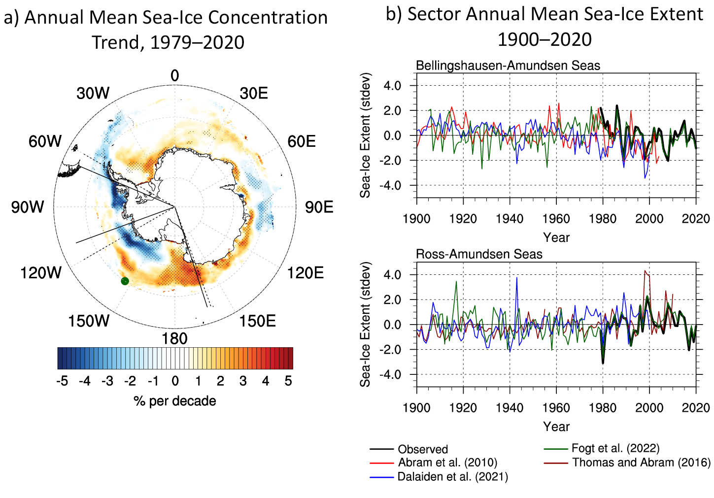 |
|
Figure 1: Sea-ice concentration trends (% per decade) from 1979-2020, with areas of stippling indicating trends that are statistically different from zero at p < 0.05. The lines denote the sectors used to define the sea-ice extent – with the dashed lines showing the sectors established by Parkinson (2019) and the solid lines sectors defined by Raphael and Hobbs (2014). (B) Timeseries of annual mean (August–October for Abram et al. 2010) standardized sea-ice extent for the Amundsen–Bellingshausen seas (top row) and Ross–Amundsen seas (bottom row). |
Nonetheless, the recent changes are captured to varying degrees by all the reconstructions, showing decreases after 1979 in the Amundsen–Bellingshausen seas, and increases in the Ross-Amundsen seas (Fig. 1b). Prior to 1979, however, there are notable differences in the average sea-ice conditions, with opposite behavior between the paleo-based and Fogt et al. (2022) reconstructions. In the Amundsen–Bellingshausen seas, the paleo-based reconstructions frequently indicate above average sea-ice extent in the early-to-mid 20th century, whereas the Fogt et al. (2022) reconstruction indicates below average sea-ice extent during this time (Fig. 1b, top). The variability is opposite in the Ross-Amundsen seas: here the paleo-based reconstructions frequently indicate below average sea-ice extent in the early-to-mid 20th century, while the Fogt et al. (2022) reconstruction indicates above average sea-ice extent prior to the onset of satellite observations (Fig. 1b, bottom). Perhaps surprisingly, the correlations with observed sea-ice concentration are all fairly similar spatially (not shown), which suggests that the various regions represented by each reconstruction is a smaller contributing factor to the disagreement in the reconstructions.
To highlight the differences further, 30-year running trends of the annual mean reconstructions are provided in Figure 2a. Notably, the paleo-based reconstructions all suggest that the sign (and often statistical significance) of the observed trends for the two regions continue throughout the 20th century. In contrast, the Fogt et al. (2022) trends indicate a change in the sign (and often statistical significance) of the trends prior to 1979.
The role of atmospheric circulation
Since Dalaiden et al. (2021) reconstructed the historical changes of the atmosphere, it is possible to also investigate changes in the atmospheric circulation in relation to sea-ice trends. Additionally, Fogt and Connolly (2021) provide another pressure dataset, which employs a seasonal, spatially complete reconstruction poleward of 60°S (Fogt et al. 2019) and the National Oceanic and Atmospheric Administration 20th-century reanalysis (Slivinski et al. 2019) equatorward of 60°S. Importantly, the Fogt and Connolly (2021) merged pressure dataset avoids large artificial trends in other datasets over Antarctica prior to 1957 and, therefore, likely provides a more robust estimate of 20th-century pressure trends (Fogt and Connolly 2021). Annual sea-level pressure trends from the two datasets are displayed in Figure 2b. In agreement with the sea-ice trends, the pressure trends from Dalaiden et al. (2021) are the same throughout the 20th century, although not statistically significant prior to 1979. In contrast, but consistent with the instrument-based sea-ice reconstructions of Fogt et al. (2022), the pressure trends in the merged pressure dataset from Fogt and Connolly (2021) show a reversal in pressure trends across Antarctica before and after 1979. Since a large portion of the Antarctic sea-ice extent in this region is driven by the atmospheric circulation, Figure 2b demonstrates that changes in the atmospheric circulation give rise to the differences between the Fogt et al. (2022) reconstructions and those derived from paleoclimatological data.
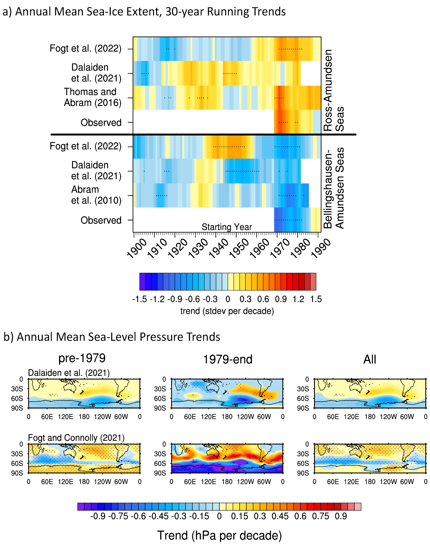 |
|
Figure 2: Thirty-year running trends of the standardized sea-ice-extent timeseries from Figure 1b. The magnitude of the trend (in standard deviations per decade) is shaded, and stippling indicates 30-year trends that are statistically different from zero at p < 0.05. (B) Annual mean sea-level pressure trends (shaded, in hPa per decade) for 1905–1979 (left column), 1979–end (middle column), and the full time period (right column). The top row is the sea-level pressure from the Dalaiden et al. (2021) simulation (which ends in 2000), and the bottom row is the merged seasonal pressure dataset (annually averaged) from Fogt and Connolly (2021), which ends in 2013. Stippling indicates trends that are statistically different from zero at p < 0.05. |
Discussion
Further work is planned to better understand the origin of these differences, with particular attention paid to the atmospheric circulation reconstruction. In contrast with the paleo-based reconstruction, the instrument-based reconstruction strongly relies on large-scale climate patterns depicted in the observations, but may not fully represent the regional and highly variable Antarctic weather that may be better captured by ice cores closer to the Antarctic sea-ice edge. Therefore, the impact of the geographical locations of the observations used in the reconstructions will be analyzed through several sensitivity experiments by including additional records, such as the near-surface air temperature and surface-pressure records from Antarctic weather stations – available since 1958 – and coral records situated in the tropical Pacific. These sensitivity experiments will aid in unlocking the contribution to regional Antarctic sea-ice variations from large-scale teleconnections, including tropical teleconnections, which have been demonstrated to play a substantial role in the Antarctic climate over the instrumental period (Holland and Kwok 2012; Meehl et al. 2016; Purich et al. 2016) on much longer timescales.
affiliations
1Department of Geography and Scalia Laboratory for Atmospheric Analysis, Ohio University, Athens, USA
2Université catholique de Louvain (UCLouvain), Earth and Life Institute (ELI), Louvain-la-Neuve, Belgium
3Fonds de la Recherche Scientifique FRS-FNRS, Brussels, Belgium
contact
Ryan Fogt: fogtr@ohio.edu
references
Abram NJ et al. (2010) J Geophys Res 115: D23101
Dalaiden Q et al. (2021) Clim Dyn 57: 3479-3503
Fogt RL, Connolly CJ (2021) J Clim 34: 5795-5811
Fogt RL et al. (2019) Clim Dyn 53: 1435-1452
Fogt RL et al. (2022) Nat Clim Chang 12: 54-62
Holland PR, Kwok R (2012) Nat Geosci 5: 872-875
Meehl GA et al. (2016) Nat Geosci 9: 590-595
Parkinson CL (2019) Proc Natl Acad Sci USA 116: 14,414-14,423
Purich A et al. (2016) J Clim 29: 8931-8948
Raphael MN, Hobbs W (2014) Geophys Res Lett 41: 5037-5045
Slivinski LC et al. (2019) Q J R Meteorol Soc 145: 2876-2908
Katherine Wilson1,2, A. Arreak1,3, Sikumiut Committee3 and T. Bell1,2
For the first time, Inuit have used their sea-ice knowledge to reconstruct historical sea-ice conditions to address climate change and resource development implications for safe sea-ice travel in their region.
The Inuit community of Mittimatalik (Pond Inlet) is located in the Canadian High Arctic (Fig. 1). Traveling on the sea ice is central to the wellbeing, identity, and culture of the Mittimatalingmiut (residents of Mittimatalik). The nearby floe edge is a highly anticipated sea-ice feature that is present from late December to early July (Fig. 1). It provides a stable, landfast, sea-ice platform to hunt and fish near the open water. Although Inuit have always experienced and adapted to variable ice conditions, changes in ice conditions are now beyond what they would consider normal (Pearce et al. 2010). Therefore, Inuit are looking for additional information to support their safe travel decision-making. However, there is a gap in the availability of current sea-ice climate products. For example, outputs from sea-ice models are not at community scale, and sea-ice charts from national ice services capture the open-water summer shipping season, and not the Inuit sea-ice travel season (November to July in Mittimatalik) (Wilson et al. 2021). With a variety of near real-time and archived satellite imagery now publicly available, Inuit training, to interpret satellite imagery and create their own maps, is the missing step to support community-based sea-ice mapping (Laidler et al. 2011; Segal et al. 2020).
Mittimatalingmiut are already dealing with the impacts of climate change on sea-ice conditions, compounded by the pressure to increase commercial shipping in early July through the sea ice to the nearby Mary River iron-ore mine and port (Fig. 1). A local committee of Inuit sea-ice experts, called Sikumiut, identified the need to document the region's historical sea-ice conditions to understand: (1) where the sea ice was becoming more dangerous, to adapt their travel routes; and (2) the potential impacts of shipping earlier to the mine. Here we describe the process of co-creating a 23-year sea-ice-change atlas (siku asijjipallianinga) with Sikumiut, how the satellite imagery and geographic information system (GIS) mapping tools and training were put in the hands of Inuit with knowledge and experience of traveling on the ice, and how the atlas differs from other products to help address Inuit priorities.
What is Sea Ice Inuit Qaujimajatuqangit?
Inuit maintain the longest unrecorded climate history of sea ice in Canada. Mittimatalik's sea-ice climatology is preserved by orally passing down this knowledge and sharing their extensive and recent travel experiences on the sea ice (called Inuit Qaujimajatuqangit, or IQ). Sikumiut's deep climatological knowledge of the seasonal evolution of sea ice is what keeps them safe while traveling on it. However, their sea-ice IQ is not in a database, but exists in the collective minds of these expert sea-ice travelers. Also, their climatology is not focused on sea-ice extent, concentration, or volume in a general scientific sense, but more specifically on ice conditions for safe travel.
Making an IQ-based sea-ice change atlas
In 2019, a pilot curriculum was developed to train Andrew Arreak, an Inuit community researcher from Mittimatalik, in satellite imagery interpretation and GIS. In 2020, Arreak interpreted over 2000 Radarsat ScanSar Wide (1997 to 2019) and MODIS (2000 to 2019) images over six weeks (18 June to 29 July) to capture the evolution of spring ice-travel conditions prior to breakup. Arreak created weekly maps to digitize areas of sea ice that were no longer safe for travel, as the warmer temperatures began to melt the snow and sea ice. Arreak's sea-ice travel knowledge, and that shared with him by Sikumiut members, allowed him to monitor known areas in the satellite imagery for rapid change due to river outflow, melting glaciers, strong ocean currents, and recurring leads (cracks that stay open in the ice). Digitized maps were converted to raster to create maps to: (1) depict average ice travel conditions for each week of breakup based on the 23-year record, and (2) capture the spatial evolution of breakup for each year. Arreak was also trained in statistical analysis to review spatial and temporal trends in the sea-ice-breakup maps.
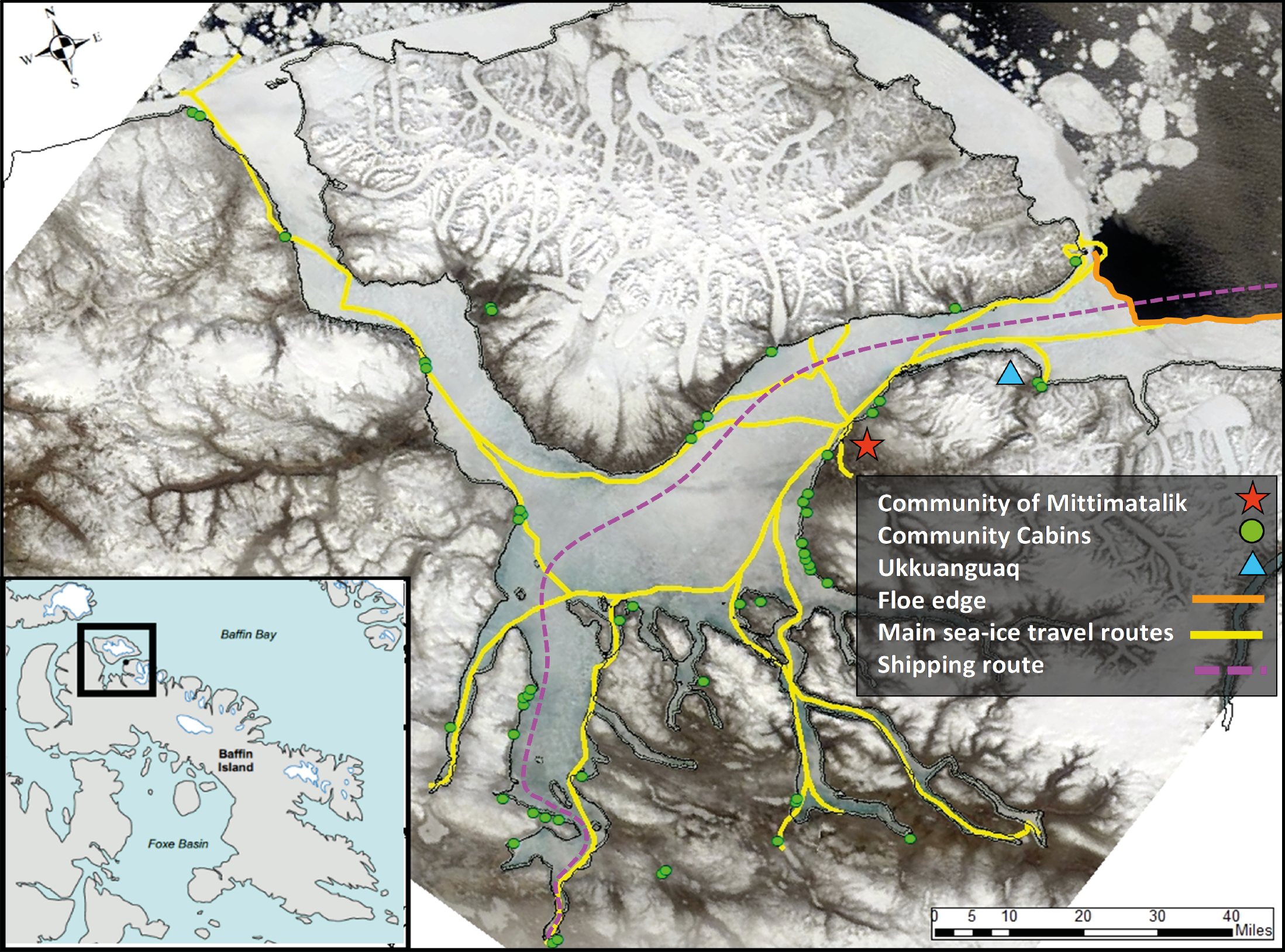 |
|
Figure 1: Map of the Mittimatalik sea ice travel region, Nunavut, Canada. Background satellite image: MODIS True Color Composite, 9 June 2019 (NASA 2019). |
What the atlas tells us about sea-ice breakup
Snowmelt on the land signals the start of the breakup season. The average onset of snowmelt in the 23-year record was detectable in the satellite imagery the week of 11–17 June. By the following week of 18–24 June, areas of open water became visible in the satellite imagery in the southeast inlets and mouths of local rivers (Fig. 2). It is normal for the floe edge to fracture and break off to form new edges during the breakup season. Areas of breakup expand in the south and southeast sounds and inlets, and along the coastlines, until travel to the floe edge is no longer safe by the week of 9–15 July. The floe edge normally breaks up the week of 16–22 July. However, there was high variability in the timing of sea-ice breakup, and only the week of 2–8 July showed a trend towards earlier breakup with an R2 value of 0.34 (p value < 0.5).
Sikumiut has discussed that the floe edge is not as stable as it has been in the past. In reviewing the satellite imagery, the normal breakup date for the floe edge was 18 July (±2 days) between 1997 and 2019. Our results show a trend towards earlier breakup (R2 = 0.42, p < 0.05) with 7 July 2019 being the earliest breakup date in the record.
Implications for safe ice travel
In 17 out of 23 years (74%), the floe edge fractured to a location called Ukkuanguaq (Figs. 1, 2). Additionally, in 16 out of these 17 years, Ukkuanguaq is the last floe-edge location before the sea ice completely breaks up. Sikumiut already knew of the significance of the Ukkuanguaq; however, this mapped evidence supports community sea-ice adaptation needs. For example, talks are already underway to position time-lapse cameras and other monitoring equipment at this location to provide Mittimatalingmiut advance notice of breakup (Bell et al. 2020).
The average patterns for where and when the sea ice becomes dangerous for travel and the evolution of breakup were consistent with Sikumiut's IQ. However, Arreak explained that in some years the sea ice in front of the community can breakup earlier than at the floe edge (Fig. 2c). To continue to hunt and fish, Mittimatalingmiut will travel overland to access the sea ice just past Ukkuanguaq. The GIS-derived summary breakup maps did not capture this pattern, so we reviewed the individual yearly maps. This type of breakup pattern occurred about half of the time (48%), and there was no apparent increase in the frequency of this pattern over the last decade. Nevertheless, given the importance of hunting at the floe edge, there have been discussions within the community to build a road to Ukkuanguaq as an adaptation strategy to maintain their hunting and fishing activities at the floe edge.
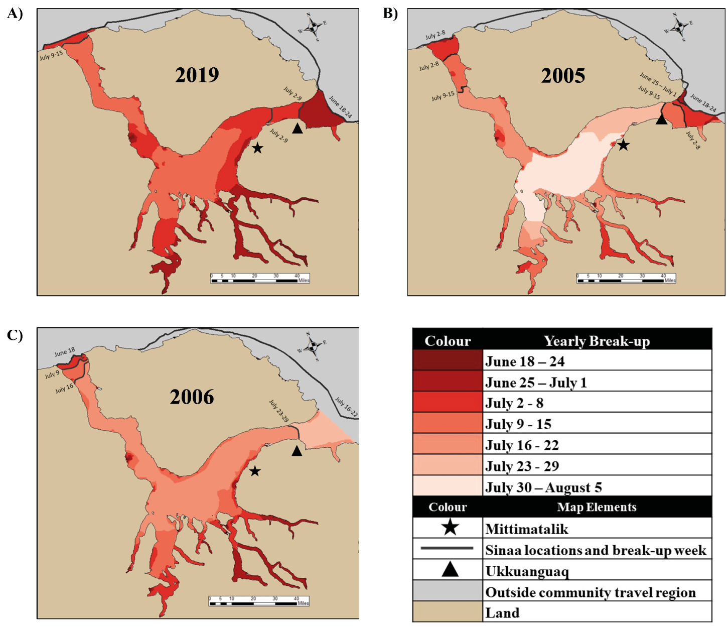 |
|
Figure 2: Yearly maps showing the spatial pattern of ice breakup in the Mittimatalik region. (A) The 2019 map shows the spatial pattern for an unusually early breakup. (B) The 2005 map illustrates the spatial pattern for an unusually late breakup. (C) The 2006 map provides an example of a year when the sea ice at the floe edge breaks last. |
The IQ-based sea-ice atlas also shows that extending the shipping season into the first two weeks of July could accelerate the breakup of the floe edge, shortening the sea-ice travel season further. If shipping is extended into the breakup season to support mining activities, Mittimatalingmiut now have a baseline of their local sea-ice conditions with which to compare and provide evidence for any future cumulative effects.
Conclusion
Siku asijjipallianinga differs from typical sea-ice climate atlases in that it used western tools to capture the collective IQ climatological sea-ice history of the region. Without Sikumiut's and Arreak's IQ and guidance, we would not have been able to interpret the satellite imagery or analyze its results from such an on-ice travel perspective. Because this atlas was created from an Inuit viewpoint, it provides an adaptation tool that Mittimatalingmiut can use to share locations of known and changing sea-ice conditions to plan for safe sea-ice travel. The atlas also clearly demonstrates the scientific merit of IQ in environmental assessments that can potentially impact the future sea-ice regime.
affiliations
1SmartICE Sea Ice Monitoring & Information Services Inc., St. John's, NL, Canada
2Department of Geography, Memorial University of Newfoundland, St. John's, NL, Canada
3Sikumiut Management Committee, Mittimatalik, Nunavut, Canada
contact
Katherine Wilson: katherine@smartice.org
references
Bell T et al. (2020) Sikumiut perspectives on monitoring ice breakup near Mittimatalik: Summary workshops report. St. John's: Unpubl. Available at SmartICE Inc. with permission
Laidler GJ et al. (2011) Can Geogr 55: 91-107
NASA (2019) EOSDIS Worldview: worldview.earthdata.nasa.gov
Pearce T et al. (2010) Polar Rec 46: 157-177