Sea level variations during the last interglacial
Mark Siddall1, R.C.A. Hindmarsh2, W.G. Thompson3, A. Dutton4, R.E. Kopp5 and E.J. Stone6
The Last Interglacial Global Mean Sea Level is believed to be 6 to 9 m above the present and might have two distinct maxima. Here, we discuss the possible fluctuations and their implications for ice sheet evolution.
The duration and timing of the Last Interglacial (LIG) Global Mean Sea Level (GMSL) fluctuations are active areas of research, with distinct features of this sea level change increasingly being reproduced in diverse datasets and syntheses (Dutton & Lambeck 2012; Kopp et al. 2009; Thompson et al. 2011). We review and discuss these possible changes in LIG GMSL and, in particular, what we may infer from them in terms of changes to continental ice.
Implications of the magnitude of the LIG GMSL maximum relative to today
Kopp et al. (2009) first synthesized a database of local sea level reconstructions for the LIG using statistically rigorous techniques within the framework of a glacio-isostatic adjustment model. They estimated that GMSL during the LIG peaked above 6.6 m (95% probability), but was unlikely to have peaked above 9.4 m (33% probability). Through an alternative deterministic approach, Dutton and Lambeck (2012) found very similar results with a range of 5.5 to 9 m. This puts LIG sea level within the window of other Quaternary GMSL maxima (± 10 m around modern sea level; Siddall et al. 2006) but places the LIG GMSL higher than most past interglacial GMSL.
The Antarctic ice sheet may have, therefore, retreated considerably during the LIG (by 0.7 to 7.6 m sea level equivalent), given the modeled estimates of the other contributing factors to sea level variations such as ocean thermal expansion and past temperature change (McKay et al. 2011), small glacier and ice cap contribution (Radić and Hock 2010) and Greenland retreat reconstructed from ice cores and ice sheet modeling (e.g. Cuffey and Marshall 2000; Lhomme et al. 2005; Otto-Bliesner et al. 2006; Robinson et al. 2011; Stone et al. 2013; Tarasov and Peltier 2003).
Although the loss of the West Antarctic Ice Sheet (WAIS) has been thought of as the most likely candidate, we cannot afford to simply assume that this is the case on the basis of potentially simplistic first-order assumptions. For example, mechanisms have been suggested which stabilize the WAIS during ice sheet retreat (Gomez et al. 2010). Even under a collapse scenario, the WAIS would be unlikely to totally disappear, instead leaving ice on land and reducing the plausible WAIS LIG sea level contribution to 3.3 m, allowing for the effects of glacial isostatic adjustment and changes in the position of the marine margin (Bamber et al. 2009). This leaves open the possibility of a reduced East Antarctic Ice Sheet (EAIS) during the LIG of up to 4.3 m. Improved understanding of sub-ice sheet topography points to this possibility (Le Brocq et al. 2010; Pingree et al. 2011) and evidence of ice rafted debris originating from zones within the EAIS has been identified for earlier periods in the Antarctic ice sheet history (Pierce et al. 2011).
Implications of the existence of two distinct GMSL maxima during the LIG
There is a suggestive similarity between the results of Kopp et al. (2009) and Thompson et al. (2011) in a period during which sea level falls and rises again by several meters over several thousand years. The fluctuation has an amplitude of 6.5±10.5 m in the GMSL reconstructions of Kopp et al. (2009) and of the order of 5 m in those of Thompson et al. (2011), in the Bahamas fossil coral terraces (which provide a self-consistent stratigraphic framework for the fluctuation). Evidence of rapid sea level changes during the LIG exists in distinct stratigraphic units, suggesting multiple reef-growth episodes (e.g. Hearty et al. 2007). However, until recently it has proved difficult to resolve the age differences between distinct reef units. Results from conventional Uranium/Thorium geochronology suggest a long, stable GMSL maximum with only a vague suggestion of any fluctuation (e.g. Stirling et al. 1998). It is certainly worth considering which mechanisms may have driven such fluctuations, if they did indeed occur (Dutton and Lambeck 2012).
We can first consider the implications of the fluctuation amplitude of the order of 5 m. Given this amplitude, we can rule out the effects of ocean thermal expansion and the global glacier budget as their respective contributions are too small to drive such a change (McKay et al. 2011; Radić and Hock, 2010). This leaves the ice sheets. We therefore examine what processes could plausibly explain a signal of this amplitude from the ice sheets and divide these into three classes:
• Contribution from the Greenland ice sheet
 |
|
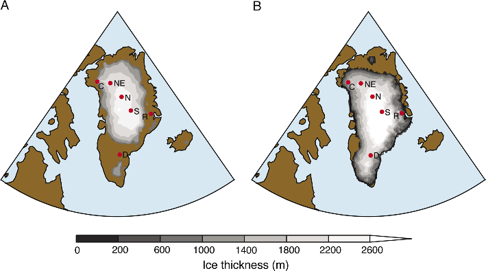
Figure 1: Simulated LIG minimum Greenland ice sheet thickness showing (A) saddle collapse from Otto-Bliesner et al. (2006) and (B) northern ice sheet retreat from Stone et al. (2013). Ice core locations are also shown: Camp Century [C], Dye-3 [D], NEEM [NE], NGRIP [N], Renland [R] and Summit [S]. Note that the presence of ice at Dye-3 may suggest that the saddle collapse mechanism was less extreme than what is shown in (A). Figure modified from Otto-Bliesner et al. (2006) and Stone et al. (2013). |
Ice sheet modeling focused on the LIG indicates substantial inland reduction of the Greenland ice sheet compared to the present (e.g. Cuffey and Marshall 2000; Otto-Bliesner et al. 2006; Robinson et al. 2011). Some of these simulations indicate a change from an ice sheet with two domes joined by a saddle to one ice sheet with two separate domes (e.g. Fig. 1A; Otto-Bliesner et al. 2006; Robinson et al. 2011) while other simulations indicate a retreat of the ice sheet in northern Greenland (e.g. Fig. 1B; Fyke et al. 2011; Stone et al. 2013). Both of these can be argued to be dynamically unstable, driven by a positive feedback. Melting of the ice represented by the saddle could, therefore, result in a fluctuation due to a rapid transition between two stable states. However, the amplitude of any saddle collapse would not be large enough to explain a sea level fluctuation as large as 5 m. Furthermore, ice sheet models have not shown yet such a rapid transition in ice volume for the LIG perhaps due to missing complex physical processes in the models.
• Contribution for the West Antarctic ice sheet
Changes to the Antarctic ice sheet would presumably occur largely at the margins in regions of sub-marine based ice, such as the WAIS or Wilkes-Aurora regions. Complete collapse of the WAIS to small ice caps in Marie-Byrd Land and Ellsworth Land is in some senses dynamically analogous to a Greenland saddle-collapse. Although this ice provides a good explanation for the high GMSL during the LIG, it is an open question as to whether grounding-line re-advance could occur sufficiently fast to initiate the sea level fall. A re-advance of the WAIS may not be an adequate explanation for GMSL fall and rise based on our present understanding.
• Contribution of both Antarctic and Greenland ice sheets
The final set of explanations refers to the phasing of the ice sheet minima in Greenland and Antarctica. Given the difference in the phasing of insolation and the plausible hemispheric asymmetry in meridional heat transfer between the poles (e.g. Stocker and Johnsen 2003), there is no special reason to assume that the ice sheet minima are coincident. There are many possible combinations of this phasing. Box 1 provides one of the more plausible scenarios.
Distinguishing these different options is a matter for future research. One key avenue will be dating the timing and duration of the GMSL maxima, because this will help elucidate mechanisms related to Northern and Southern Hemisphere insolation. Another key avenue will be exploiting geographic patterns in sea level change, combined with sedimentary observations near ice sheets, to constrain changes in different ice sheet volumes over the LIG. More observations to better constrain the magnitude of the sea level oscillation will be critical to help discern the potential ice sheets involved. Finally, additional suggestions that GMSL during the LIG peaked more than twice (Rohling et al. 2008; Thompson et al. 2005; Thompson et al. 2011) would require more creative thinking in terms of understanding the mechanisms driving these persistent oscillations.
Oppenheimer et al. (2008) define the concept of "negative learning" in the following terms: "New technical information may lead to scientific beliefs that diverge over time from the a posteriori right answer". Whatever the story really is, evidence for high, fluctuating GMSL during the LIG must leave us with very open minds regarding ice sheet behavior to avoid the past traps of "negative learning" when it comes to past and future changes in ice sheets.
Box 1: One possible scenario for evolution of the Greenland and Antarctic ice sheets during the LIG.
The following terms are defined as:
GrIS: Greenland Ice Sheet
AIS: Antarctic Ice Sheet
EAIS: East Antarctic Ice Sheet
GMSL: Global Mean Sea Level
WAIS: West Antarctic Ice Sheet
STAGE 1 - The GrIS reaches its minimum first and the AIS has partially retreated (for example, the EAIS is reduced compared to today). GMSL reaches its first peak.
STAGE 2 - The GrIS begins to regrow and the AIS remains partially retreated. GMSL falls.
STAGE 3 – The GrIS continues to regrow but the AIS retreats more quickly (for example the WAIS reduces). GMSL rises.
STAGE 4 – The AIS begins to regrow (now in phase with the GrIS) and the glacial inception commences. GMSL falls.
acknowledgements
This discussion largely came out of the PALSEA PAGES workshop held at University of Wisconsin, Madison in June 2012 (this issue, p. 40). We are grateful to Bette Otto-Bliesner for providing the results shown in Fig. 1A.
affiliations
1Department of Earth Sciences, University of Bristol, UK mark.siddall@bristol.ac.uk
2Science Programmes, British Antarctic Survey, Cambridge, UK
3Department of Geology and Geophysics, Woods Hole Oceanographic Institution, Woods Hole, USA
4Department of Geological Sciences, University of Florida, Gainesville, USA
5Department of Earth & Planetary Sciences and Rutgers Energy Institute, Rutgers University, New Brunswick, USA
6School of Geographical Sciences, University of Bristol, UK
Selected references
Full reference list online under: pastglobalchanges.org/products/newsletters/ref2013_1.pdf
Dutton A, Lambeck K (2012) Science 337: 216-219
Kopp RE et al. (2009) Nature 462: 863-867
Le Brocq AM, Payne AJ, Vieli A (2010) Earth System Science Data 2: 247-260
Oppenheimer M, O’Neill BC, Webster M (2008) Climatic Change 89: 155-172
Thompson WG, Curran HA, Wilson MA, White B (2011) Nature Geoscience 4: 684-687