New perspectives on the isotopic paleothermometer

Mathieu Casado and Anaïs J. Orsi

> Access contents of this issue

> Download this article as pdf

Past Global Changes Magazine

31(2)

100-101

2023

https://doi.org/10.22498/pages.31.2.100

Mathieu Casado

1 and Anaïs J. Orsi

1,2

Water isotopes in ice-core records are often used as a proxy of past temperature variations. Their use is based on an empirical relationship which requires care to limit the impact of the multiple contributions to the isotopic signal.

Water isotopes in ice-core records are a favored proxy of past temperature variations (Dansgaard 1964). The isotopic signal is formed by the distillation of the heavier isotopes during the advection of moist air masses from the oceanic areas, where evaporation takes place, to the precipitation sites in polar regions (Fig. 1a). As such, the temperature signal of precipitation integrates all the changes of temperatures along the pathway, following the geophysical fluid dynamic (Bailey et al. 2019). In addition, the isotopic signal is modulated by the precipitation intermittency at the ice-core drilling site (Casado et al. 2020; Münch et al. 2021), the local exchange between the snow and the atmosphere (Steen-Larsen et al. 2014; Wahl et al. 2021), the redistribution by the wind and its interactions with the local stratigraphy (Fisher et al. 1985), and snow metamorphism and diffusion inside the snow (Casado et al. 2021).

Isotopic composition of precipitation

Historically, the link between isotopic composition and temperature was assessed by spatially correlating the concurrent change of temperature and isotopic composition across Greenland and Antarctica (Dansgaard 1964). This spatial correlation was then used to convert isotopic records from ice core to past temperature records (Stenni et al. 2004) and supported by models ranging from simple Rayleigh models (Ciais and Jouzel 1994) to isotope-enabled global coupled models (iso-GCM) (Werner et al. 2018).

In a pure Rayleigh distillation model, the isotope-temperature relationship is dictated by the temperature control of the rainout fraction, under a moist-adiabatic framework (i.e. following the Clausius-Clapeyron law) (red dots in Fig. 1b). Using the spatial relationship between isotopic composition and temperature to predict the temporal relationship (space for time analogy) would work if the moisture pathways always remained the same, and the spatial gradients of isotope and temperature were evaluated directly over these moisture pathways. In reality, each precipitation event is associated with the advection of moisture air masses with different origins in terms of distance, temperature and humidity conditions (blue dots in Fig. 1b). This leads to the isotope-to-temperature relationships varying with space, time, and timescales, which is not reproduced by Rayleigh models. Yet, Rayleigh models are still heavily used for their simplicity compared to more complex models, such as iso-GCM which have shown the limits of the space-for-time analogy at timescales ranging from seasonal to multi-millennial (Werner et al. 2018). Newer distillation models using a moist-isentropic framework (i.e. not following Clausius-Clapeyron, but instead keeping the potential temperature constant) remain easy to use, and they can explain more features, such as the difference between spatial and temporal slopes (Bailey et al. 2019).

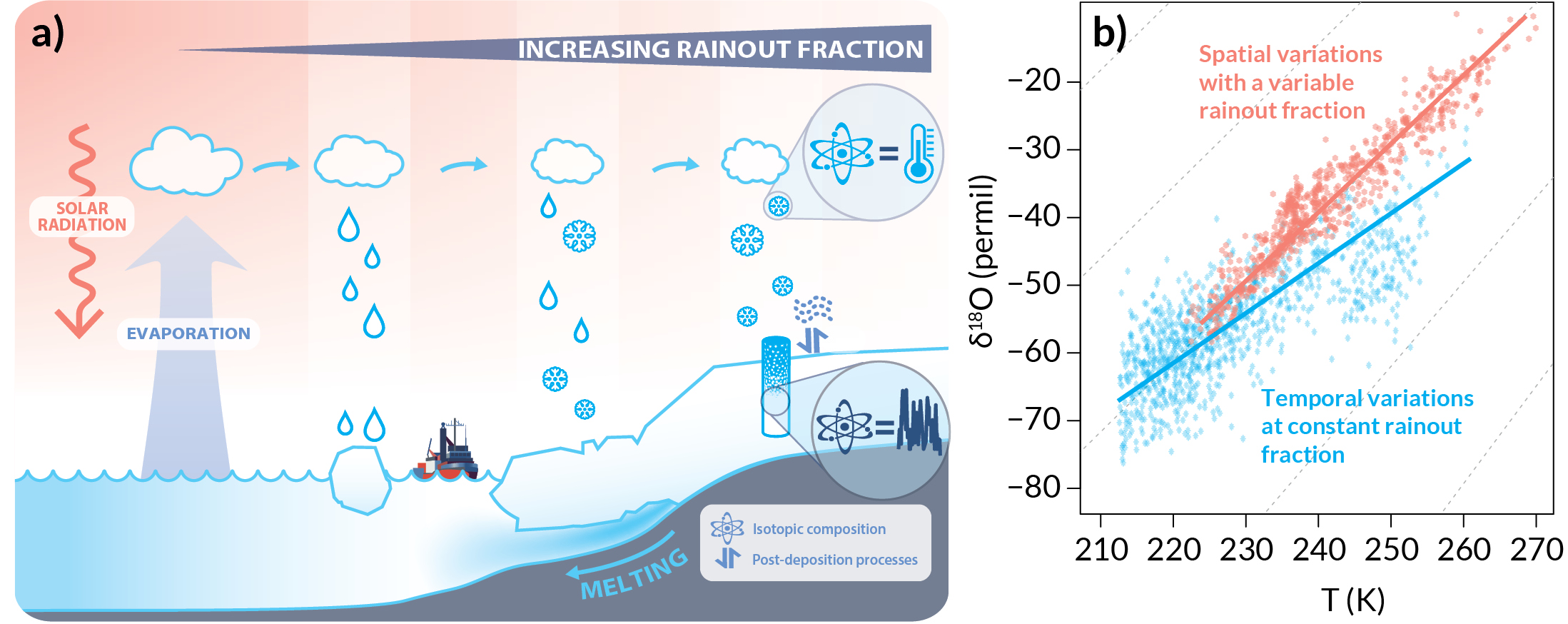Figure 1: (A) Schematics of the acquisition of the isotopic signal in ice cores: Rayleigh distillation and diffusion; and (B) variations of isotopic composition as a function of temperature, across spatial gradients (red), and across temporal changes (blue).

Archiving of the signal in the snow

As the signal is only recorded when snowfalls occur, the precipitation intermittency creates a significant modulation of the recorded signal (Casado et al. 2020). Overall, the aliasing of the seasonal cycle by precipitation intermittency creates a white noise contribution which can be more than 10 times stronger than the climatic signal at interannual and decadal scales. This can be easily visualized using the power spectral density, i.e. the amount of energy that is included in the signal at a given frequency, which shows that the peak associated to the seasonal cycle (Fig. 2a) is redistributed across frequencies (dashed blue arrows in Fig. 2b). In glacial times, winter precipitation is suppressed, which causes an under-estimation of temperature change. This effect is particularly clear during stadial–interstadial cycles in Greenland (Guillevic et al. 2013). In modern times, interannual variability in precipitation is driven by the presence of extreme events in winter (Servettaz et al. 2020). The diagnostic of precipitation intermittency is important for the analysis of each ice-core record. Isotope-enabled global climate models are the tool of choice to quantify the relationship between atmospheric circulation patterns and the precipitation water-isotope composition. The relatively small spatial footprint (100–200 km) of precipitation events can also be used to design an optimal array of cores to average out the precipitation noise (Münch et al. 2021), and mitigate the impact of precipitation intermittency.

After the snow has been deposited, it can remain exposed near the surface for a long period of time, especially in low accumulation areas. This leads to a wide range of further alterations of the isotopic signal. Most interactions between the snow and the atmosphere, such as wind redistribution (Fisher et al. 1985), and sublimation and condensation (Casado et al. 2021; Wahl et al. 2021), also induce an aliasing of the signal, and create more white noise with a common structure of a few meters only (Münch et al. 2016). Inside the firn, snow metamorphism (Casado et al. 2021) and isotopic diffusion tend to lead to a low pass filtering of the signal, removing the high frequency variability (solid blue arrow in Fig. 2b). The impact of stratigraphic noise can be mitigated by stacking cores from a few meters apart, thanks to the very short decorrelation length of the noisy component. The diffusion effects can be numerically removed when the measurement noise is sufficiently low (Casado et al. 2020).

Limits of the isotopic paleothermometer

The variable isotope-temperature relationship, as well as these archival processes, limit the possibility for an absolute isotopic paleothermometer. Indeed, the temperature signal which can be simulated by a red noise signal (Fig. 2a), undergoes the conversion into isotopic units (green curve in Fig. 2b), and then is heavily affected by diffusion and archival noises (blue solid curves in Fig. 2b). All these effects make it arduous to obtain a calibration by matching the isotopic signal with times series obtained from weather stations (Fig. 2c; Osborn and Briffa 2004). In addition, as weather stations at ice-core study sites (Antarctic, the Arctic, high mountain regions) usually have very short record length, and under the influence of climate change, the variability against which the isotopic signal is matched does not correspond to natural variability. Overall, even with a “perfect” independent calibration, if the noisy contributions are not removed, the variability is only well estimated at low frequency (Fig. 2d).

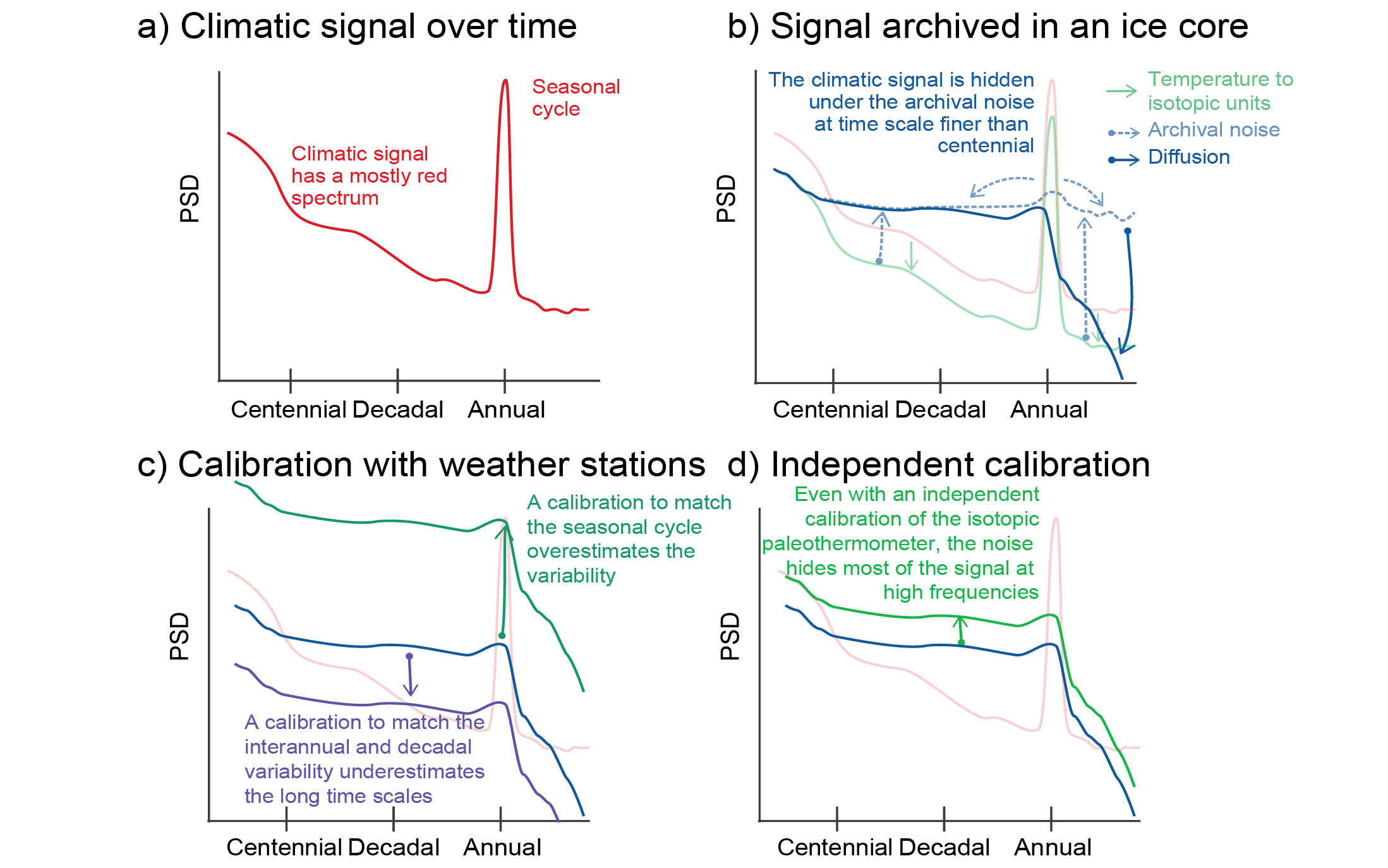Figure 2: Description of the isotopic paleothermometer calibration through the power spectral density (PSD) at different timescales (centennial, decadal and annual) showing: (A) climatic signal spectrum; (B) alteration of the isotopic signal (solid blue line) compared to the climatic signal during archival processes; (C) calibration against short, recent temperature records at annual and decadal timescales; and (D) independent calibration that does not match the variability at a given scale, but does not remove the noise from the signal before the climatic reconstruction (inspired from Osborn and Briffa 2004 and Casado et al. 2020).

Conclusion

Although the interpretation of water isotopes remains challenging, there are exciting new developments in the interpretation of water isotopes in ice-core records beyond the linear isotopic paleothermometer. Comparing the different noisy components amongst several ice cores can provide information on past precipitation patterns, as well as on the wind conditions and the surface roughness. Combining several isotopic compositions (d-excess, 17O-excess) also expands the scope of reconstructions from water isotopes, including the latent heat fluxes at the surface and within the firn (Casado et al. 2021). Infrared spectrometry offers new possibilities for high-resolution measurements in ice cores to study in situ post-depositional processes in the snow and in the water vapor. Better measurements will support updated trajectory models, isotope-enabled global climate models, and proxy system models, making water isotope science an expanding field of research.

affiliationS

1Laboratoire des Sciences du Climat et de l’Environnement, CEA–CNRS–UVSQ–Paris-Saclay–IPSL, Gif-sur-Yvette, France

2Department of Earth, Ocean and Atmospheric Sciences, University of British Columbia, Vancouver, Canada

contact

Mathieu Casado: mathieu.casado@gmail.com

references

Bailey A et al. (2019) Geophys Res Lett 46: 7819-7827

Casado M et al. (2020) Clim Past 16: 1581-1598

Casado M et al. (2021) Geophys Res Lett 48: e2021GL093382

Ciais P, Jouzel J (1994) J Geophys Res 99: 16793

Dansgaard W (1964) Tellus 16: 436-468

Fisher DA et al. (1985) Annal Glaciol 7: 76-83