PAGES Magazine articles
Organic compounds in ice cores are valuable tracers of past terrestrial and marine biospheres. Analytical challenges have previously prevented quantification of these compounds, but recent breakthroughs have allowed us to measure and better understand biogenic processes and past atmospheric circulation.
Organic tracers in the cryosphere
Important paleoclimatic information can be yielded from the analysis of organic impurities in ice cores. Organic compounds contribute up to 90% of total fine aerosol particle mass. Thus, they contain large amounts of information about the sources and transport patterns of aerosols (Kanakidou et al. 2005). Organic particles and microorganisms can be cloud condensation and ice-nucleating particles, which means they can easily end up being deposited as snow. Additionally, wet precipitation is an efficient scavenger of organic particles from the atmosphere. Ice cores serve as an archive of the past atmosphere since they contain traces of organic aerosol particles and dissolved organic matter. Despite this, very few organic compounds have been successfully quantified in ice cores. Biomass burning tracers, such as levoglucosan and vanillic acid, and the sea-ice proxy methanesulfonic acid, are examples of organic compounds which have been successfully quantified in ice cores.
Challenges with quantification of organic compounds in ice
The greatest challenge with quantification of organic compounds in ice cores is their low concentrations. The total organic carbon content in ice cores from Antarctica has been measured in several ice cores to be between 5 and 900 ppb carbon (Federer et al. 2008; Legrand et al. 2013), which results in individual compounds being found at ppb or ppt levels. Most analyses of organic compounds in ice cores, therefore, require preconcentration steps. Ice cores are cut into discrete samples and the exposed outside is removed with a knife before the ice is melted and often preconcentrated. Preconcentration is the process of increasing the concentration of target compounds in a sample, either by collecting the target compounds from the solution, or by evaporating the solvent from the mixture. Preconcentration improves detection, but often part of the target compound is lost in the process. The amount of initial substance preserved after the preconcentration steps is referred to as the “recovery rate”. Preconcentration methods used for organic compounds in ice have reported recovery rates upwards of 80% (King et al. 2019; Müller-Tautges et al. 2014). However, with discrete ice-core samples, the spatial resolution is limited as these methods often require high sample volumes. A measurement of the recovery rate of each compound measured is also necessary for proper quantification. Additionally, the process is labor intensive and the repeated cutting of the ice cores risks sample losses.
Preunkert et al. (2011) found that lab air could be a significant source of organic carbon contamination in their melted ice samples due to the dissolution of atmospheric traces of formic and acetic acids. These authors found a rapid increase in dissolved organic carbon (DOC) in open bottles of ultrapure water left in a clean room and in a “general purpose” room. The general purpose room had a contamination increase two orders of magnitude higher than in the clean room. Even a closed bottle in the general purpose room was found with a 25 ppb carbon DOC increase per hour, but this was much lower than the approximate 3000 ppb carbon DOC increase per hour observed in the open bottle, in the same location. This demonstrates that great care is needed to limit contamination of samples, especially after cutting and melting discrete samples of ice. One way of preventing this issue is by omitting the sample preparation steps altogether. This can be done using continuous methods, rather than discrete samples.
Continuous sampling and measurements of ice cores
Continuous flow analysis (CFA) has become one of the standard methods of ice-core analysis since it was developed in the 1990s (Fuhrer et al. 1993; Sigg et al. 1994). In CFA, sticks of ice are melted from the bottom, and the meltwater is continuously pumped into instruments for analysis. The sample experiences little to no contact with air, and is directly analyzed a few seconds after melting (Fig. 1). The melthead is often shaped so only the innermost section of ice is directed to the most sensitive analyses. The outermost ice is used for analyses less prone to contamination, such as stable water isotopes (δ18O and δD). CFA reduces several of the issues related to analyzing organic compounds, such as airborne contamination and sample losses from cutting the ice. The drawback is that contamination can stem from the tubing, and signals may be dispersed in the tubing due to diffusion processes (Rasmussen et al. 2005).
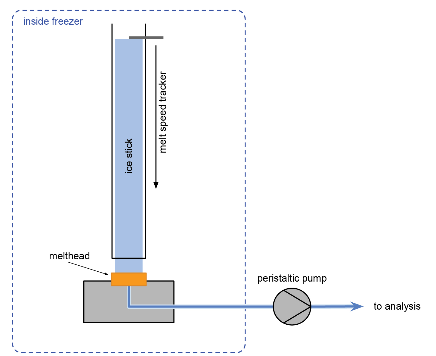 |
Figure 1: Continuous flow analysis (CFA) melting system. Ice cores are cut into sticks, which are placed on the melthead. The melt speed is regulated through the temperature of the melthead. Peristaltic pumps direct meltwater from the melthead to instruments for analysis. |
The greatest challenge still is that very few methods are able to detect compounds at the low concentrations found in ice cores with high time resolution. Shi et al. (2019) measured discrete surface-snow samples in Antarctica, and observed mean concentrations of vanillic acid and syringic acid of 5.74x10⁻² pg/mL and 3.84x10⁻² pg/mL, respectively (1 pg = 10–12 g).
Barbaro et al. (2022) recently coupled a CFA melter to a fast liquid chromatography tandem mass spectrometer (FLC-MS/MS). They quantified vanillic and syringic acids, and recently also levoglucosan in alpine ice cores. The method uses two liquid chromatography columns in parallel, allowing one column to be in use while the other is flushed and prepared for the next sample. This results in fast measurements with a spatial resolution of 1 cm. The methods’ limit of detection (LOD) was 3.6 pg/mL and 4.8 pg/mL for vanillic acid and syringic acid, respectively (Barbaro et al. 2022). Comparing the LOD of this method to the concentrations found in Antarctic snow shows that current methods involving CFA are not yet able to quantify organic compounds in Antarctica, but can be useful in areas with higher concentrations of organic trace components, such as continental glaciers.
Factors influencing observed organic components in ice
Measurements of organic compounds in ice have given us insight into biomass burning, sea-ice extent in the Antarctic, and anthropogenic pollution in the past (Fig. 2). Continental glaciers can yield more local information, while ice cores drilled on ice sheets in Antarctica or Greenland can serve as atmospheric background pollution levels.
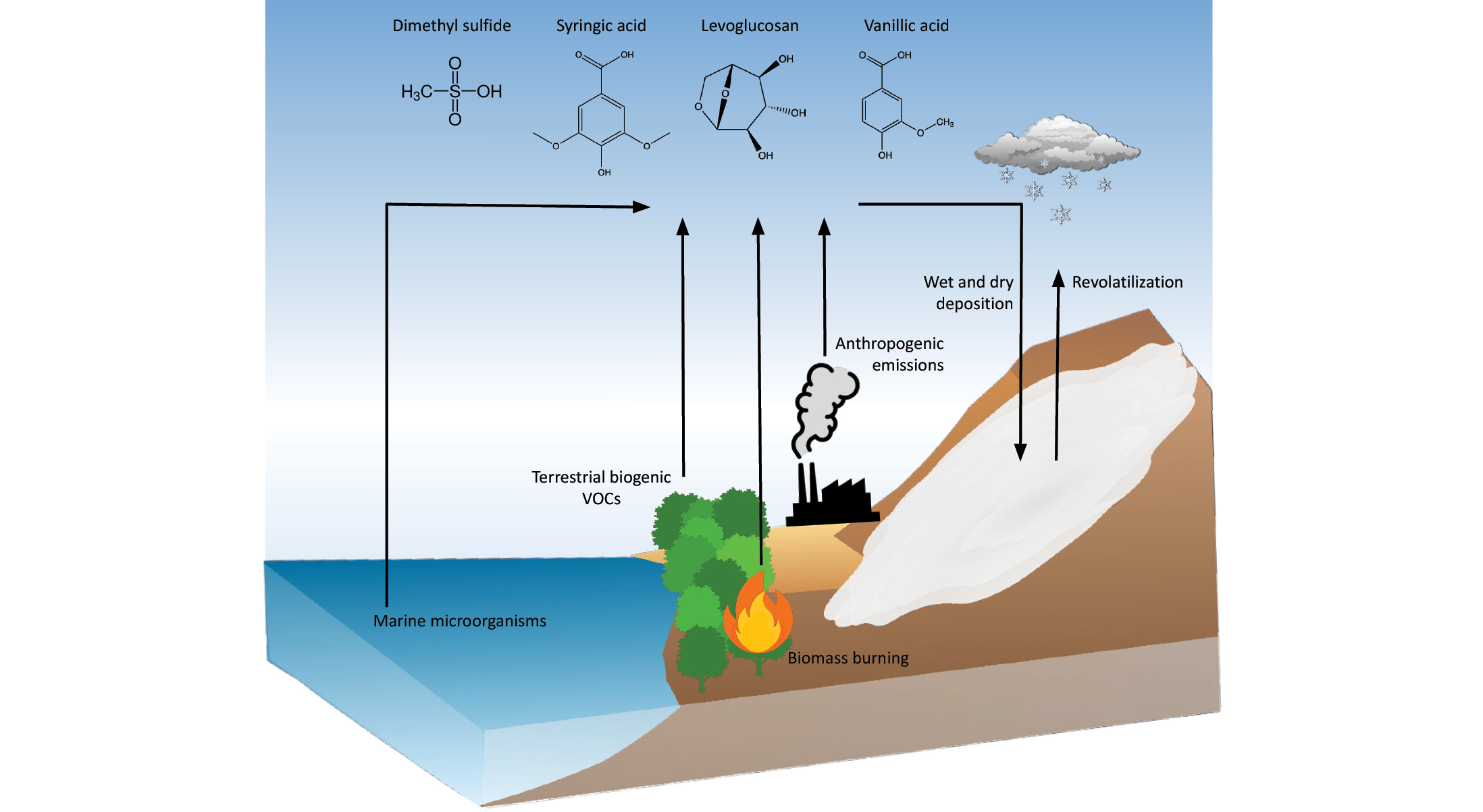 |
Figure 2: Schematic of transport pathways from sources such as marine microorganisms, terrestrial vegetation, wildfires, and anthropogenic emissions to glaciers and ice sheets. The organic compounds can be deposited as dry or wet deposition, and after deposition, compounds can be chemically or biologically degraded or revolatilized to the atmosphere. |
Shi et al. (2019) found higher levels of levoglucosan and syringic acid near the Antarctic coast compared to further inland. They found no trend with distance from the coast for vanillic acid. Since the compounds have the same sources and similar chemical structures, it is expected that levoglucosan and syringic acid are more sensitive to oxidation and are consequently depleted more rapidly in the atmosphere than vanillic acid. The oxidation of compounds must, therefore, be taken into consideration when interpreting measurements from ice cores. Industrial and fossil-fuel-related emissions have increased the oxidative potential of the atmosphere (Lelieveld and Dentener 2000), which could disproportionately deplete the signal of organic compounds in recent centuries of ice-core chronologies. For older sections of ice, post-depositional effects, such as chemical and microbial degradation, UV-induced degradation in the surface snow, and revolatilization of compounds, must be considered. These post-depositional effects are not currently well understood, but could have differing effects on the levels of organic compounds in different layers of ice.
Conclusion
Organic compounds remain largely unexplored in ice cores, mainly due to difficulties with contamination and not having sensitive-enough methods. Recent developments have allowed continuous measurements of organic biomass burning tracers in alpine ice cores, and high-resolution measurements of discrete ice samples from Antarctica. Methods are being improved to increase both the number of organic analytes being measured in one core, and the temporal resolution of the ice-core chronology. By analyzing fatty acids, terpenes, phenolic acids, and other components, we gain insight into the terrestrial and marine biospheres of the past, as well as anthropogenic impact on atmospheric chemistry. Developing analysis methods further will allow us to unveil more of these processes, and better understand the biogenic processes and atmospheric circulation in the past.
affiliation
1Institute for Marine and Atmospheric Research, Utrecht University, The Netherlands
contact
Hanne Ø. Notø: h.o.noto uu.nl
uu.nl
references
Barbaro E et al. (2022) Anal Chem 94: 5344-5351
Federer U et al. (2008) Environ Sci Technol 42: 8039-8043
Fuhrer K et al. (1993) Atmos Environ Part A Gen Top 27: 1873-1880
Kanakidou M et al. (2005) Atmos Chem Phys 5: 1053-1123
King ACF et al. (2019) Talanta 194: 233-242
Legrand M et al. (2013) Clim Past 9: 2195-2211
Lelieveld J, Dentener FJ (2000) J Geophys Res 105: 3531-3551
Müller-Tautges C et al. (2014) Anal Bioanal Chem 406: 2525-2532
Preunkert S et al. (2011) Environ Sci Technol 45: 673-678
Rasmussen S et al. (2005) J Geophys Res Atmos 110: 163-169
The Asian deserts were identified as the primary source of mineral dust in Greenland ice. However, secondary sources may be overlooked when quantifying contributions of different sources in large bulk samples. Single particle studies can help overcome these limitations.
How mineral dust is archived in Greenland ice
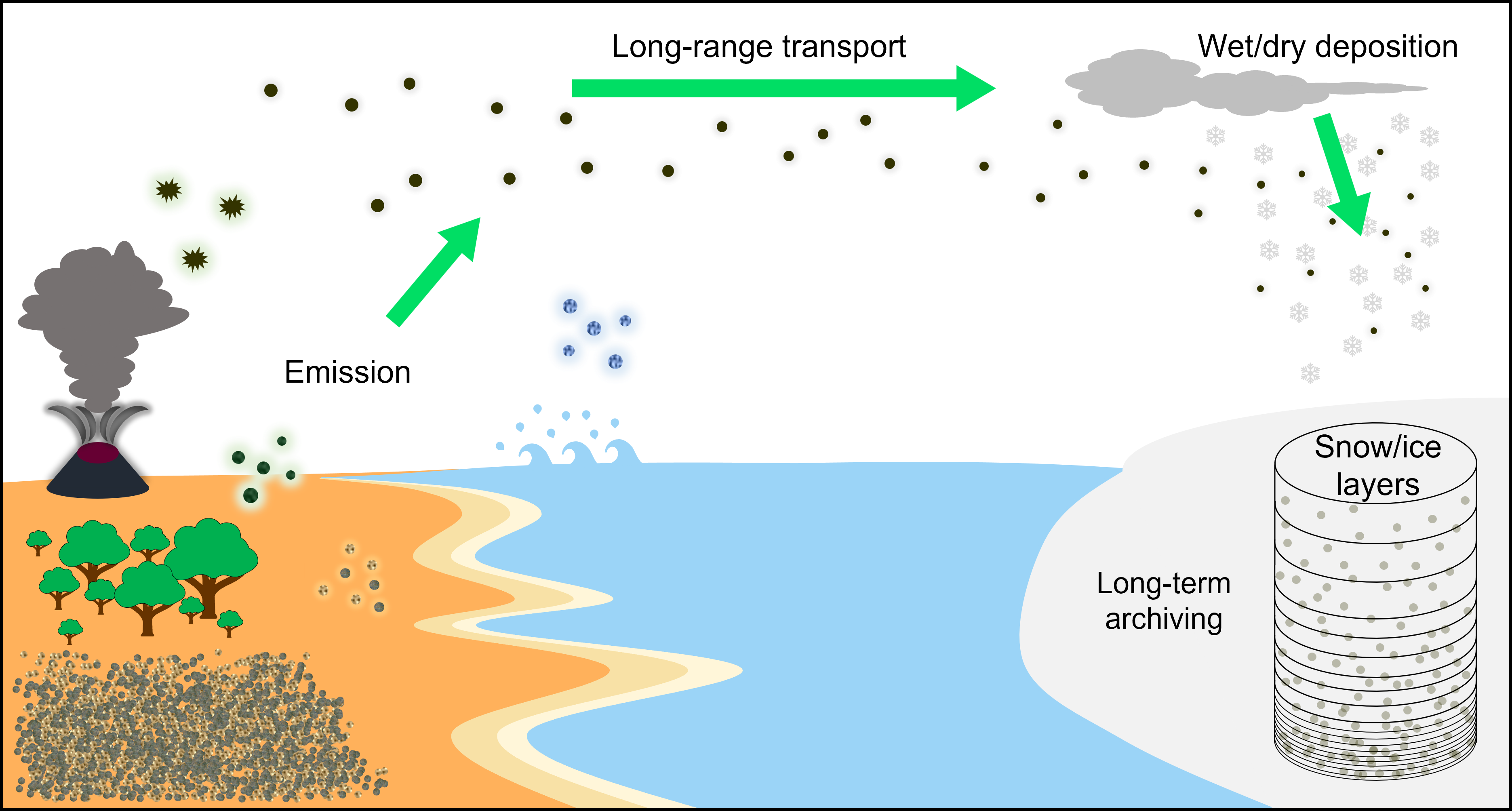
Various types of aerosols are produced in different environments on Earth. For example, volcanoes emit aerosols and precursor gases during their eruptions, oceans generate sea-salt aerosols, and deserts produce mineral dust aerosols (Fig. 1). Among these aerosols, mineral dust plays a crucial role in aerosol composition.
|
|
Figure 1: Life cycle of aerosol components archived in ice cores. Aerosol species are emitted from various sources, such as deserts, vegetation, volcanic activities, and oceans, and then transported over long distances by atmospheric circulation. Aerosols (such as dust) are wet- and dry-deposited en route and onto the ice sheet, and preserved in ice layers. |
The emission of soil-derived dust into the atmosphere occurs when the wind velocity is high enough to disperse the dust. The threshold wind velocity depends on the particle size, mass, and soil moisture content in the source region. In quantitative terms, the flux of dust generated by the wind is nonlinearly dependent on wind speed (Marticorena and Bergametti 1995). Reconstructing the strength of dust emission from measured ice-core concentrations can help us understand climate change in the source regions.
Many of the major dust sources are located in arid regions of the extratropics due to their dry and windy conditions. This restricted location of dust sources implies that dust must be transported over long distances by atmospheric circulation to reach Greenland. The atmospheric lifetime of dust depends on its size, mass, and the degree of washout by precipitation en route. Thus, climatic changes, such as alterations in atmospheric circulation patterns and precipitation, impact the transport efficiency of dust to Greenland. Long-range transported dust is deposited onto the surface of the Greenland Ice Sheet through both wet and dry processes. Size-dependent dry deposition of aerosols always occurs, whereas wet deposition can only occur if a precipitation event happens on the ice sheet. In summary, for efficient dust export to the Greenland Ice Sheet, dry and windy conditions at the source region and little precipitation en route are necessary (which typically implies transport at high altitudes). Ideally, precipitation over the ice sheet should occur at the time the dust plume reaches Greenland.
Different approaches to determine where the mineral dust came from
Various methods have been used to investigate the sources of dust in Greenland ice. Satellite imagery has been used to observe the transport of dust from its sources to Greenland directly. For example, Prospero et al. (2002) used satellite pictures to identify the desert belt extending from North Africa to Eastern Asia as the primary source of dust in the Northern Hemisphere. Since satellite imagery can only be obtained from cloud-free scanned regions and only for the last few decades, it falls short of providing a comprehensive understanding of the influence of past climate on the sources of dust in Greenland ice.
Atmospheric circulation modeling also enables the exploration of dust transport also for past and future conditions. Kahl et al. (1997) modeled back trajectories of air masses from Summit Station, Greenland. They found that approximately 60% of all winter trajectories to Summit, Greenland, were connected to a cluster that allows for aerosol transport from the East Asian desert dust source region, whereas a cluster connected to the North American dust source region was dominant (46%) in summer. However, this approach has limitations in accurately determining the source apportionment when atmospheric conditions are poorly defined in the model. This is especially true for past climate conditions that cannot be validated against meteorological observations, compromising the accuracy of the model’s results in such cases.
Direct analysis of the dust deposited onto the Greenland Ice Sheet is another effective way to determine its origin. Mineralogy, elemental composition, and isotopic composition are widely used (often in combination) for source identification. Mineralogy can help identify the type of soil using crystal information. For example, Maggi (1997) characterized the mineralogical composition of dust from glacial and interglacial periods in the Greenland Ice Core Project ice core and compared it with dust samples from low- and high-latitude source regions. The results suggest that warm periods are characterized by a higher contribution from chemical weathering in low-latitude source regions compared to more mechanical weathering in mid-latitudes during cold periods.
The elemental and isotopic composition of dust can serve as unique fingerprints for identifying dust sources, and are typically measured using mass spectrometry. Bory et al. (2003) used the mineralogy and isotopic signatures of the dust in snow-surface samples to identify present-day dust sources for Greenland. The mineralogical signatures found in all the dust samples from Greenland snow pits, characterized by low kaolinite to chlorite ratios, provide clear evidence that the sources are dominated by East Asian desert areas. This finding rules out North America and Northern Africa as major sources (Bory et al. 2003). The isotopic signatures of the samples not only agreed with the East Asian origin determined by their mineralogy, but also showed pronounced seasonal variation in sources within Asian inland regions. The Taklamakan Desert contributes substantially to the dust transported to northern Greenland during the maximum dust concentration in spring, while the main source of dust for autumn is shifted to the Tengger and Mu Us deserts (Bory et al. 2003).
However, some recent studies have suggested that the sources of dust may be more complex than previously thought, and may vary in response to abrupt climatic changes, such as Dansgaard-Oeschger events (Han et al. 2018; Újvári et al. 2022).
Single particle analysis: A new approach to dust characterization
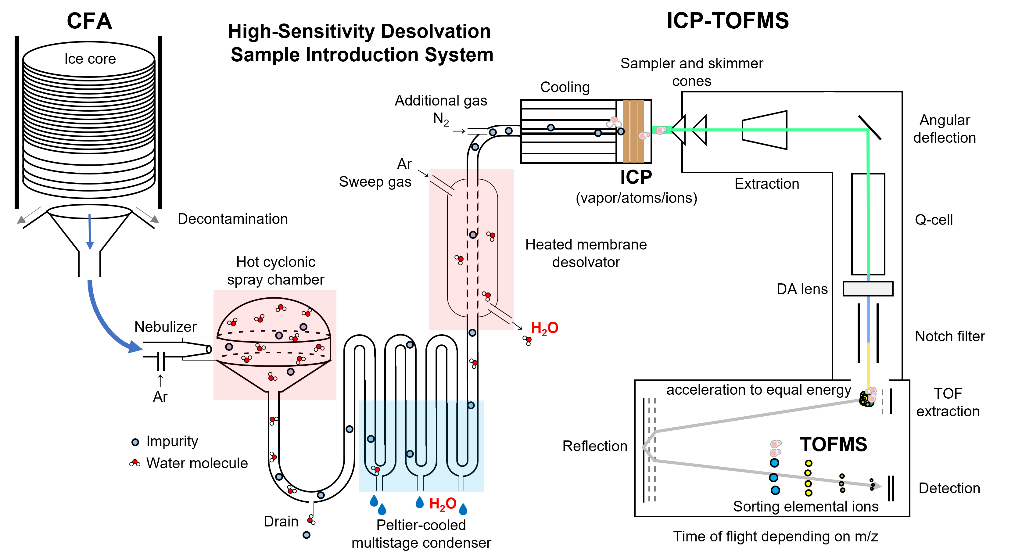
Most of the aforementioned chemical methods which describe bulk parameters of large ice samples after melting and pretreatment, like acid digestion, have inherent limitations. This implies that (i) chemical characterization by these methods cannot distinguish between particulate and dissolved dust tracers and (ii) bulk samples average a mixture of many individual dust particles which may originate from different source regions. To overcome these limitations, we follow a new approach that takes advantage of the millisecond time resolution of single-particle inductively coupled plasma time-of-flight mass spectrometry (sp-ICP-TOFMS) (Fig. 2). This novel approach enables the detection and elemental characterization of single dust particles in addition to the dissolved impurities in a meltwater stream provided by the continuous flow analysis (CFA) developed at the University of Bern (Kaufmann et al. 2008). First results on the elemental composition of single dust particles from Greenland meltwater samples support Asian deserts as the main origin of the long-range transported particles to Greenland (Erhardt et al. 2019).
Conclusions and outlook
The origin of dust in Greenland has been determined through various approaches, such as remote sensing, atmospheric circulation modeling, and direct measurements of dust in ice cores. Many previous studies, using diverse approaches, agree that Asian deserts are the primary sources of dust transported to central Greenland. However, we stress the importance of high-resolution single dust particle analysis (Erhardt et al. 2019), in addition to bulk analysis. The sp-ICP-TOFMS enables the investigation of elemental composition of individual dust particles in samples. This allows the precise characterization of the fingerprints of individual soil-derived aerosols from both source samples and Greenland ice, including the internal variation within each source region and source mixing.
Within the DEEPICE project, we are furthering these studies by improving our analysis system with a desolvation sample introduction, which dries the sample stream before it enters the plasma (Fig. 2). Drying the sample helps to reduce loss of analytes during the introduction, and minimizes spectral interferences caused by the input of water into the system. Furthermore, we are developing automated data analysis routines to characterize different clusters of dust origin. However, diverse methods should be used complementarily to improve our understanding of the origin of dust in Greenland ice under different climatic conditions.
|
|
Figure 2: Schematic diagram of CFA-sp-ICP-TOFMS with a high-sensitivity desolvation sample introduction system. The meltwater sample from the CFA flows into the desolvation unit and undergoes a drying process through heating, condensation, and membrane diffusion during sample introduction. The ions reaching the TOFMS can be analyzed over the 23 to 254 mass range, and due to the high time-resolution of sp-ICP-TOFMS, individual dust particles can be detected, in addition to the dissolved background. |
affiliations
1Climate and Environmental Physics, Physics Institute and Oeschger Centre for Climate Change Research, University of Bern, Switzerland
2Alfred Wegener Institute, Helmholtz Centre for Polar and Marine Research, Bremerhaven, Germany
contact
Geunwoo Lee: geunwoo.leeunibe.ch
references
Bory AJM et al. (2003) Geophys Res Lett 30: 1167
Erhardt T et al. (2019) Environ Sci Technol 53: 13275-13283
Han C et al. (2018) Sci Rep 8: 15582
Kahl JD et al. (1997) J Geophys Res: Oceans 102: 26861-26875
Kaufmann PR et al. (2008) Environ Sci Technol 42: 8044-8050
Maggi V (1997) J Geophys Res Oceans 102: 26725-26734
Marticorena B, Bergametti G (1995) J Geophys Res Atmos 100: 16415-16430
Prospero JM et al. (2002) Rev Geophys 40(1): 1002
Újvári G et al. (2022) J Geophys Res Atmos 127: e2022JD036597
Diffusion of water molecules in ice cores attenuates high-frequency variability of the water-isotope records, strongly affecting the interpretation of the deepest, oldest ice. Our ability to partly restore the signal depends on the measurement noise and our knowledge of the diffusion length.
Water-isotope diffusion
Stable water isotopes (δ18O and δD) stored in ice sheets serve as a valuable proxy of the climate at the time of deposition as snowfall. However, over time, the water isotopes disperse, either between the porous snow and surrounding air at the top of the ice sheet (Whillans and Grootes 1985), or through other processes such as solid-ice-bulk diffusion (Johnsen 1977; Ramseier 1967) or liquid-water veins (Nye 1998) once the snow has been compacted into ice. This process is known as diffusion and attenuates the isotopic signal, primarily over the higher frequencies (shorter timescales), causing a smoothing effect. The degree of attenuation is characterized by the diffusion length, which is the average displacement of water molecules from their initial position within the ice sheet. Since this is a cumulative effect, ice thinning increases the affected timescale as the ice layers descend. Additionally, the very deepest ice close to bedrock is warm, reaching temperatures close to the pressure melting point. This greatly increases the diffusion length due to the non-linear dependence of the ice-diffusivity coefficient on temperature. Consequently, variability on centennial and even millennial timescales can be reduced significantly by diffusion in very old ice. Typical diffusion lengths in the firn range from 0–15 cm (Gkinis et al. 2021; Johnsen et al. 2000), while in the deep ice some estimates suggest values up to 60 cm (Pol et al. 2010). Knowledge of the diffusion length is important, as it enables us to determine on which timescales climate variability is preserved, and even restore some of the attenuated signal.
How diffusion affects the water-isotope signal
To visualize the potential effect of diffusion on the water-isotope signal in deep ice, we produced a virtual water-isotope record with the properties of the Beyond EPICA Oldest Ice Core (BE-OIC) currently being drilled in Antarctica. As an assumed climate record, we use the marine benthic stack (Lisiecki and Raymo 2005, "LR04 stack"), a landmark climate record based on a global collection of δ18O measurements in benthic foraminifera. This record represents global ice volume and is strongly correlated on glacial-interglacial scales with Antarctic ice-core records. We adjust the age scale of this record to an age-depth model (Chung et al. 2023) of the BE-OIC, and rescale and invert the benthic δ18O values using the EPICA Dome C δ18O record (EPICA community members 2004), taking the peak of the Last Interglacial Period and Last Glacial Maximum as reference points.
As an example of the potential effect of diffusion, we zoom into a 25 m section in the deep part of this virtual ice core that represents 11 glacial–interglacial cycles from 1.2 Myr BP to 1.6 Myr BP (Fig. 1a). Simulated diffusion was applied to the record using three different diffusion lengths, demonstrating the potential magnitude of the smoothing effect. While a diffusion length of 10 cm (blue) simply rounds out the sharp peaks and troughs, a diffusion length of 60 cm (red) greatly attenuates the amplitude of even the glacial–interglacial cycles.
To quantify this effect, we calculate the remaining variability of a given frequency as the diffusion length is increased (Fig. 1b). We show the remaining power at decamillennial timescales (light gray, 10 kyr), as well as the dominant frequency driving glacial–interglacial variability both before (dark gray, 41 kyr) and after (black, 100 kyr) the Mid-Pleistocene Transition (MPT) (Clark et al. 2006). Significant decamillennial variability only remains for a diffusion length of 10 cm, while on the 100-kyr timescale less than a third of the power is lost, even for a 60 cm diffusion length. The glacial–interglacial cycles in Figure 1a mostly follow a 41-kyr cycle trend, represented by the dark gray curve in Figure 1b. The striking difference in the smoothing of this glacial–interglacial variability for different diffusion lengths is intuitive, once compared with the three diffusion lengths marked on the 41-kyr curve. While approximately 94% of the power remains when diffused with a 10 cm diffusion length, less than 11% survives once the diffusion length is increased to 60 cm.
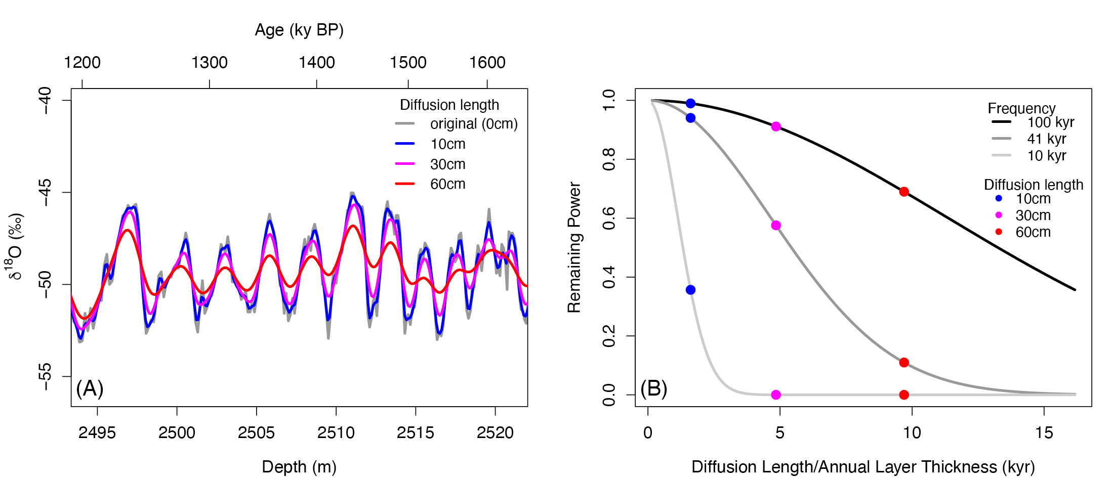 |
Figure 1: (A) Effect of diffusion length on the simulated deep ice-core record. (B) Remaining power at specific timescales against diffusion length in time units, converted from depth units by dividing by the average annual layer thickness across the depth range shown in (A). The three frequencies represent decamillennial variability (light gray, 10 kyr), Earth’s obliquity cycle, dominant before the MPT (dark gray, 41 kyr) and Earth’s eccentricity cycle, dominant after the MPT (black, 100 kyr). The colored dots represent the diffusion lengths shown in (A). |
Recovery of the water-isotope record
For a better reconstruction of past climate evolution, we would like to be able to recover some of the diffused information. To achieve this, we need to know how much variability has been lost at every frequency. Thus, we need to know the diffusion length. It is possible to statistically estimate the diffusion length by analyzing the power spectrum of a water-isotope record. Using the spectral representation of diffusion outlined in Johnsen et al. (2000) enables us to apply a fit to the power spectrum of the water-isotope record to empirically derive the diffusion length (Fig. 2a).
Once a diffusion length has been obtained, we are able to back-diffuse the isotope record through a process called deconvolution. This technique amplifies the variability of the diffused frequencies to the expected initial amplitude, reversing the smoothing process. If water-isotope measurements were taken flawlessly, with perfect precision and no noise introduced by sampling preparation, handling and analytical uncertainty, then it would be possible to almost perfectly reconstruct the signal originally archived in the upper firn layers. In practice, measurement noise is a significant limiting factor for deconvolution. At the highest, most diffused frequencies, this noise often greatly exceeds the remaining climate signal. Amplifying these frequencies will also blow up the noise, destroying the signal. To resolve this, we can filter out the frequencies with a signal-to-noise ratio (SNR) below one, through the use of a Wiener filter (Wiener 1949). As we are losing the fastest variations, the recovered signal is still smoother than the original, undiffused LR04 stack record (Fig. 2b).
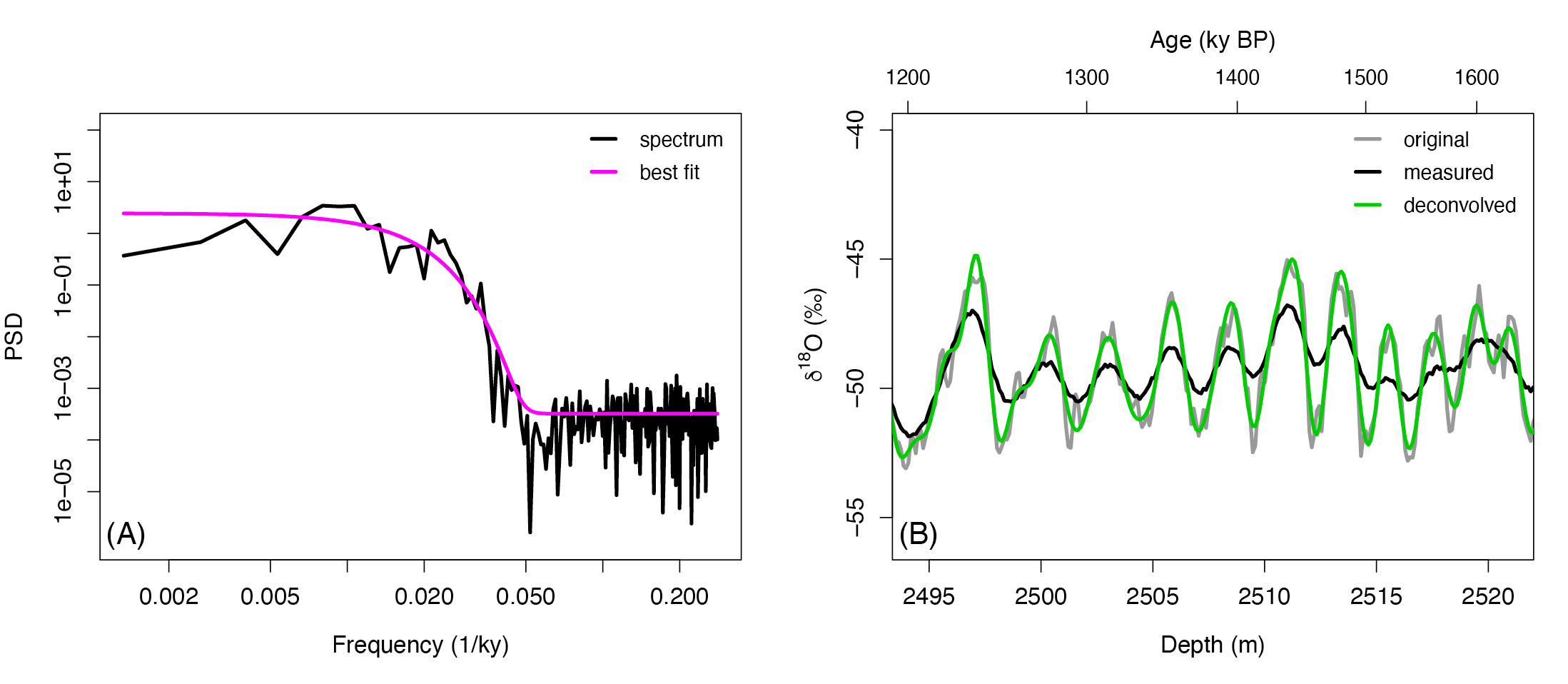 |
Figure 2: (A) Power spectrum of the diffused virtual isotope record from Figure 1a, assuming 60 cm diffusion and noise (black) and best fit (magenta). (B) Time series of the 60 cm diffused record (black) and deconvolved using Wiener deconvolution (green). Also shown is the original record before diffusion (gray). The amplitudes of the original glacial–interglacial cycles are restored, but with negligible sub-millennial variability remaining. |
In addition to minimizing the measurement noise, it is also important to obtain an accurate diffusion length, in order to calculate the magnitude of attenuation for each frequency, and to correctly identify at which frequency the SNR drops below one. Deconvolving with an incorrect estimate will either over-amplify lower frequencies if the diffusion length is too large, or amplify the higher noisy frequencies if the diffusion length is too small. Therefore, improvements to diffusion–length estimation methods and models are indispensable for high–quality signal reconstructions of this kind.
Summary
The loss of high–frequency variability in water-isotope records due to diffusion in ice cores poses a significant challenge when attempting to infer past climate. This problem is especially pronounced in deep ice cores where, due to densification and geothermal heat flux, layers are extremely thin and much warmer in the deepest, oldest ice. Statistical methods exist for estimating the diffusion length, which can be used not only to better interpret these smoothed water-isotope records, but also restore variability across certain attenuated timescales. Improved reliability and effectiveness of deconvolution techniques is possible through refining diffusion-length estimation methods, and optimizing measurement processes to minimize the measurement noise. It is also crucial for obtaining as much information as possible from future deep ice-core projects.
affiliationS
1Alfred Wegener Institute, Helmholtz Center for Polar and Marine Research, Potsdam, Germany
2MARUM – Center for Marine Environmental Sciences and Faculty of Geosciences, University of Bremen, Germany
3Physics of Ice, Climate, and Earth, Niels Bohr Institute, University of Copenhagen, Denmark
contact
Fyntan M. Shaw: fyntan.shawawi.de
references
Clark PU et al. (2006) Quat Sci Rev 25: 3150-3184
EPICA community members (2004) Nature 429: 623-628
Gkinis V et al. (2021) J Glaciol 67: 450-472
Lisiecki LE, Raymo ME (2005) Paleoceanography 20: PA1003
Nye JF (1998) J Glaciol 44: 467-468
Pol K et al. (2010) Earth Planet Sci Lett 298: 95-103
Ramseier RO (1967) J Appl Phys 38: 2553-2556
Whillans IM, Grootes PM (1985) J Geophys Res Atmos 90: 3910-3918
Due to thinning of ice-core layers, the deepest part of the cores is the hardest to analyze. New micro-destructive and high-resolution instrumental approaches are necessary to retrieve a water-isotope record that accurately represents past climate variations.
Water isotopic composition of ice cores
When water travels from the evaporation to the precipitation site, the different water isotopes (H216O, H218O, HD16O) modify its isotopic signature, represented by δ18O and δD. For example, a lighter isotope, such as H216O, evaporates more easily than a heavy one, such as H218O, leading to a temperature-dependent fractionation and the establishment of a relationship between water isotopic composition and condensation temperature (Dansgaard 1953).
Ice cores exhibit distinctive layered characteristics where the water-isotopic signature is preserved. Due to the preservation of ice for long time periods in large ice sheets, water-isotope data offers access to a continuous and high-resolution record of past climatic variability. This is shown in the climate records generated during the EPICA (1996–2008) deep-core project which extend up to 800,000 years ago. The ongoing Beyond EPICA (2019–2026) project aims to extend the ice-core record up to 1.5 Myr in order to reconstruct Antarctica’s climate history.
However, analyzing deep ice cores poses challenges. Thinning of annual layers in the deeper sections of an ice sheet, and post-depositional processes within the ice core, such as water molecule diffusion within the ice, may result in the smoothing of the water-isotope signal (Johnsen et al. 2000). This challenges the recovery of the original isotopic signal of the deposited precipitation. In addition, there are limitations in the measurement procedures which further increase difficulty in retrieving the original climate signal.
Analytical techniques for water-isotope measurements on ice cores
Advances in sample preparation and signal acquisition techniques have significantly enhanced the capability of obtaining high-resolution water-isotopic data from ice cores. Isotope Ratio Mass Spectrometry (IRMS) is an analytical technique traditionally employed to acquire water-isotope signals that offer high-precision measurements. However, due to the “sticky” nature of the water molecule, and its condensable gas phase, the water should be converted into a chemical form that is compatible with the IRMS, which is a time-consuming process and prone to inaccuracies. Laser-based water-isotope measurement techniques display the potential to tackle the aforementioned issues (Kerstel and Gianfrani 2008), as well as other difficulties related to the expensive and bulky instrumental equipment needed.
Cavity Ring Down Spectroscopy (CRDS) is a sensitive spectroscopic technique that uses laser light and an optical cavity to measure water-isotope ratios. For the measurement, a laser pulse is injected into an optical cavity, and the decay time, or "ring down" time, of the detected light intensity is measured. This decay time is affected by the presence of gas molecules in the cavity, indicating the gas concentration. By coupling specific laser wavelengths with absorption features of the target molecules, CRDS allows for highly sensitive measurements.
CRDS has emerged as a preferred alternative to IRMS, also offering the ability to perform field measurements. Different ice-sample preparation methods enable water-isotope measurements using a CRDS analyzer in either continuous or discrete mode, respectively. However, it is important to note that both approaches require substantial time and sample consumption.
Laser Ablation: a fast micro-destructive sampling method
Laser-matter interaction has been widely used for developing new techniques, including micromachining, laser cutting, sampling, and material development. When a pulsed laser beam is focused on a target surface, a high amount of energy is confined in space and time in the irradiated area, which can cause material ejection in the gas phase, known as Laser Ablation (LA). Ice sampling using LA serves a dual purpose: 1) It provides high-resolution analysis, and 2) it uses the smallest amount of sample possible for analysis, given the micro-destructive nature of the ablation process. In this way, the ice core is not melted and the same sample can be used for other types of analysis while, at the same time, it is possible to obtain high-quality continuous measurements.
LA has already been adopted as a sampling method in elemental concentration studies on ice cores (Della Lunga et al. 2017). Recently, LA sampling allowed for fast two-dimensional imaging of the impurities in ice at very high resolution (just a few tens of micrometers), generating new insights into ice-impurity interactions (Bohleber et al. 2021).
Laser Ablation–Cavity Ring Down Spectroscopy on ice cores
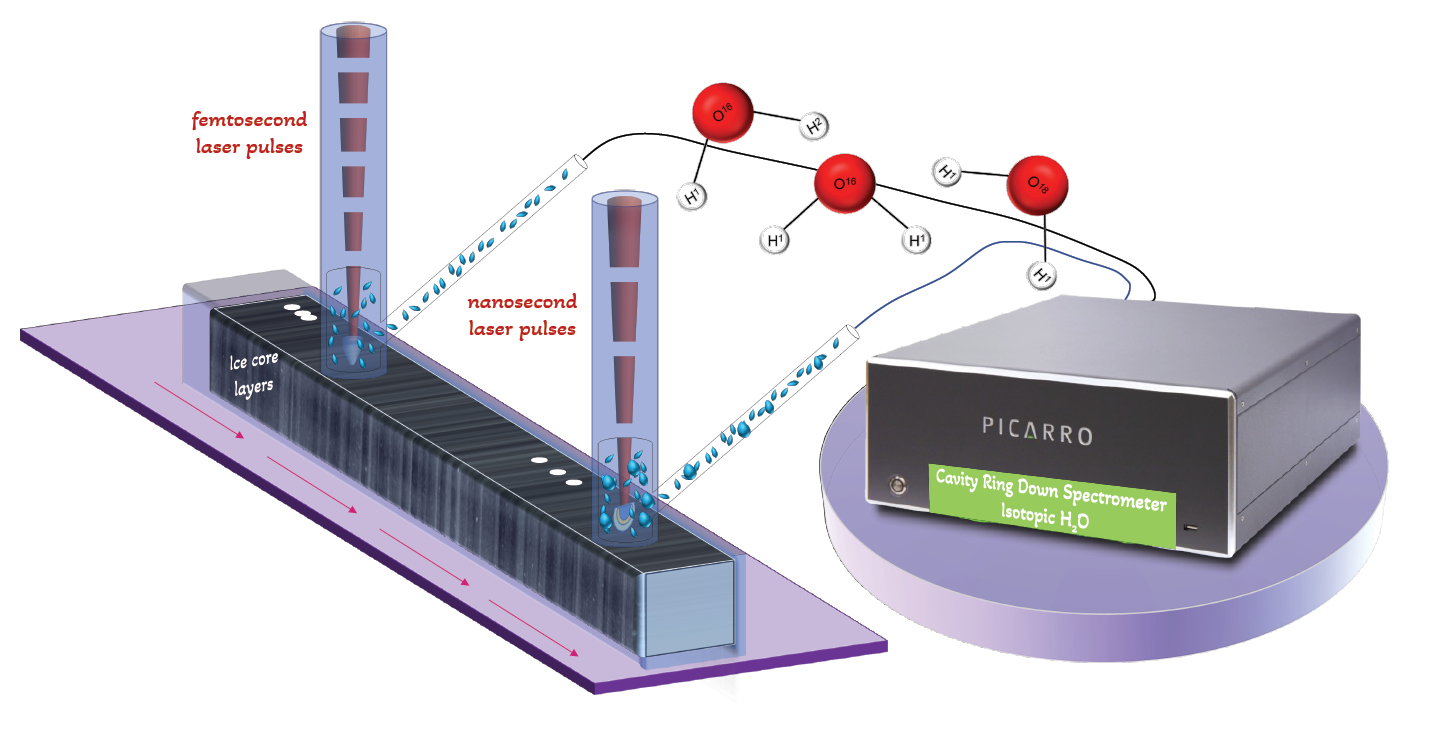
Laser Ablation (LA) and Cavity Ring Down Spectroscopy (CRDS) techniques have recently been used together to enable high-quality water-isotopic measurements on ice cores. The conceptual design of the LA-CRDS system is illustrated in Figure 1. The experimental setup for LA sampling on ice includes essential components such as a focused laser beam, a motorized translational stage for accurate ice movement, an ablation chamber to collect the sampled material, and a transfer line that transports it to the CRDS analyzer. These components work together to enable efficient and reliable analysis of ice samples in a continuous manner.
|
|
Figure 1: LA on ice-core samples using either nanosecond or femtosecond laser pulses enable material ejection in the gas phase, which is delivered to a CRDS analyzer for water-isotope detection. Placing an ice sample on a motorized stage can enable continuous high-resolution sampling. |
During sampling, the laser interacts with the ice and creates a mixture of vapor and tiny particles. The laser can produce short pulses, either in the nanosecond or femtosecond range. The amount of time the laser interacts with the ice affects the composition of the mixture. One challenge in measuring water isotopes is that when the ice melts or undergoes incomplete phase changes, it can change the isotopic signature of the material being studied. However, using very short laser pulses in the femtosecond range can help reduce this issue, because the interaction time is shorter than the time it takes for heat to spread in the material.
The compatibility between the vapor produced by the LA sampling process and the gas analyzer, CRDS, led to the inception of the LA-CRDS technique. This innovative design enables fast gas-phase sample collection directly from the ice, facilitating high-quality water-isotopic measurements. The successful implementation of this approach in experimental laboratories has yielded promising results.
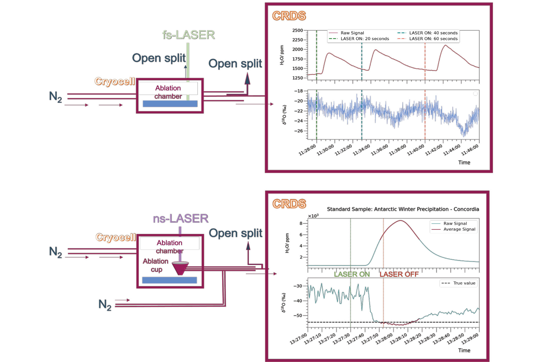
Both femtosecond (Fig. 2a; Kerttu 2021) and nanosecond laser pulses (Fig. 2b) have been applied in two distinct experimental configurations coupled with a CRDS analyzer, leading to the detection of the ablated ice (artificial ice samples produced from purified and liquid water from Antarctic winter precipitation) and acquisition of the respective water-isotope signal. These initial results demonstrate the feasibility of ablating ice material with lasers of different pulse durations, and acquiring a water-isotope signal using the CRDS analyzer.
|
|
Figure 2: (A) LA-CRDS scheme using femtosecond laser pulses and a cryocell as the ablation chamber (Kerttu and Gkinis 2021). (B) LA-CRDS scheme using nanosecond laser pulses and a two-volume cryocell (ablation chamber and ablation cup). Both LA schemes led to ice ablation. The resulting vapor, H2O, and the corresponding isotopic signal δ18Ο detected by the CRDS analyzer, are shown in both cases. |
Conclusions
Advances in water-isotope measurement techniques, both on the sampling and the detection side, had already shown a big impact on the retrieval of continuous high-resolution water-isotope records from ice cores. By combining precise analyzers with melting methods, scientists can obtain detailed data.
The introduction of LA, coupled with CRDS analyzers, presents a promising approach for capturing high-resolution isotope signals, especially from the deepest parts of the ice cores. This micro-destructive technique minimizes sample usage while providing valuable insights into laser-ice interaction principles for accurate interpretation of the water-isotope instrumental signal. The synergistic work on diffusion studies (Gkinis et al. 2014; Holme et al. 2018), and the development of high-quality water-isotope measurements, will further enhance the precision of past-temperature estimations.
affiliationS
1Physics of Ice, Climate, and Earth, Niels Bohr Institute, University of Copenhagen, Denmark
2Department of Environmental Sciences, Informatics, and Statistics, Ca’Foscari University of Venice, Italy
contact
Eirini Malegiannaki: eirini.malegiannakinbi.ku.dk
references
Bohleber P et al. (2021) The Cryosphere 15: 3523-3538
Dansgaard W (1953) Tellus 5: 461-469
Della Lunga D et al. (2017) The Cryosphere 11: 1297-1309
Gkinis V et al. (2014) Earth Planet Sci Lett 405: 132-141
Holme C et al. (2018) Geochim Cosmochim Acta 225: 128-145
Johnsen S et al. (2000) Phys Ice Core Rec 121-140
Kerstel E, Gianfrani L (2008) Appl Phys B Lasers Opt 92: 439-449
Kerttu MP (2021) MSc Thesis, University of Copenhagen, 46 pp
Stable water-isotope records from Antarctic ice cores allow the reconstruction of past temperature variability. However, accurate interpretation of the isotopic signal requires comprehensive understanding of the processes leading to its archiving in snow and ice, which can be documented by in situ measurements.
In the history of paleoclimate research, Antarctic ice cores have been largely used to unveil past variability of the Earth’s climate. As an example, the EPICA ice core drilled at Dome C in East Antarctica provided the longest record of past atmospheric conditions up to 800,000 years back in time (EPICA community members 2004). Within the ice matrix of the cores, the stable water isotopes are traditionally used as a proxy for past local temperatures. This is based on the observed correlation between the local atmospheric temperature and the surface snow δ18O across spatial transects in Antarctica (see review by Masson-Delmotte et al. 2008 and references therein).
A first challenge to the interpretation of isotopic records of snow and ice is related to the large-scale dynamics of the water cycle that vary through time, but are well constrained in global climate models (e.g. Cauquoin and Werner 2021). Along their trajectory from evaporation to precipitation onto the ice sheet, the air masses reaching the interior of the Antarctic continent are modified by precipitation and sublimation of snow that modulates the isotopic composition of the water vapor. In addition, on the East Antarctic plateau, snow accumulation is the result of a few precipitation events often associated with warm-air intrusions (Genthon et al. 2016). This leads to a discontinuous and temperature-biased recording of the stable water-isotope signal in the accumulating snow.
The ability to infer past temperatures from ice cores is also based on the assumption that the precipitation isotopic composition is preserved from snowfall to deeper burial in the snowpack. However, post-depositional processes taking place at the snow–atmosphere interface have been identified to modify the snow isotopic composition after precipitation. At Dome C, the daily-to-seasonal variations observed in the snow isotopic composition cannot be explained by precipitation only, demonstrating the existence of further processes involved in the formation of the snow isotopic signal (e.g. Casado et al. 2018).
Surface processes
At the ice sheet’s surface, the snow is affected by three kinds of physical processes: (i) wind redistribution of the snow; (ii) water-vapor exchanges between the snow and the lower atmosphere; and (iii) diffusion of water vapor within the snow. At very dry and low accumulation sites, such as the East Antarctic Plateau, the snow is exposed for long periods of time before being isolated from the influence of the atmosphere. During these precipitation-free periods, the first two processes mentioned above play a role in the resulting isotopic signal found in the snow.
A large variety of meteorological conditions are encountered on the plateau, but because of its location high up on the ice sheet, and the very small local slope, Dome C is not affected by strong katabatic winds (Genthon et al. 2021). Nevertheless, surface winds are sometimes strong enough to erode and redistribute the snow (Libois et al. 2014), which causes an inhomogeneous distribution of the water isotopes at the surface.
The surface snow and the atmosphere above also exchange moisture through sublimation of snow or condensation of water vapor onto the surface (Fig. 1). The direction and magnitude of these moisture fluxes are driven by temperature and humidity gradients between the snow and the atmosphere, while wind enhances the mixing process. Although sublimation was previously thought to be a process that did not modify the snow isotopic composition, recent studies have challenged this assumption. Steen-Larsen et al. (2014) first demonstrated the existence of water-vapor exchange between the snow and the atmosphere during summer in Greenland, leading to variations in the isotopic composition of the snow, even in the absence of precipitation bringing fresh snow to the surface. Further measurements confirmed the impact of moisture fluxes on the snow isotopic composition (Wahl et al. 2021).
Diffusion, on the other hand, is a process continuously taking place inside the snowpack. At the grain scale, in the porous space of the snow below the surface, the ice crystals sublimate and the vapor is transported and re-deposited onto other snow grains (Fig. 1). This results in the movement of water molecules driven by temperature and isotopic gradients inside the snowpack, affecting the isotopic composition of the snow and firn after snowfall (Casado et al. 2021; Johnsen et al. 2000).
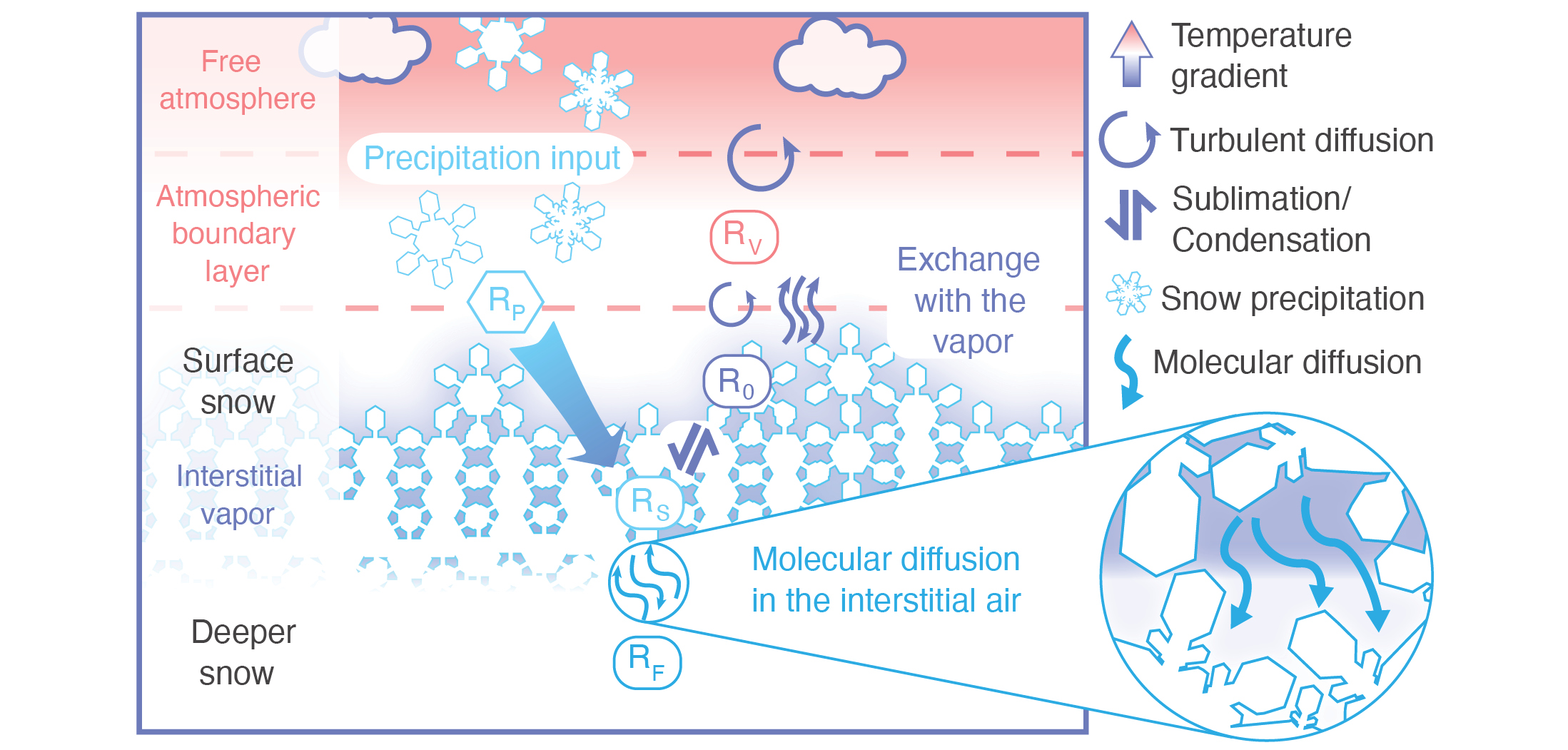 |
Figure 1: Contribution of the different reservoirs to the isotopic composition of the snow. R stands for the isotopic composition of the vapor (RV), vapor at equilibrium with snow (R0), precipitation (RP), snow (RS) and firn (RF). The two water vapor transport mechanisms are mapped: sublimation/condensation at the surface, and molecular diffusion within the snow. Figure modified from Casado et al. (2018). |
In situ observations
To provide observational benchmarks for isotope-enabled climate models, and to improve the understanding of post-depositional processes at the surface, measurement campaigns have been carried out for several years at Dome C.
The recent development of laser spectrometry has made it possible to measure the water-vapor isotopic composition in a very dry atmosphere. At Dome C, the analyzer installed on site (PICARRO L2130i) has provided observations of the atmospheric water-vapor isotopic composition almost continuously since November 2018 (Casado et al. 2016; Leroy-Dos Santos et al. 2021). The results obtained during the summer month of December 2018 are shown in Figure 2. The existence of diurnal cycles in the near-surface vapor isotopic composition (blue line in Fig. 2), following the diurnal cycles exhibited by the atmospheric temperature (orange in Fig. 2), demonstrates the existing link between these two atmospheric parameters. In addition, the analyzer recorded the atmospheric river event (a narrow corridor of intense moisture transport) that occurred between 18 and 26 December. This event led to ambient temperatures up to -15°C, which is much warmer than the average daily mean temperature of -31°C typically observed at this time of the year (Genthon et al. 2021). During this event, the vapor isotopic composition also increased by about 10‰, possibly due to a shift in the source region of the air mass, or less distillation along the trajectory from the source to Dome C.
Besides the atmospheric measurements, samples are regularly taken in the field to monitor the snow isotopic composition. In December 2018, the snow and atmospheric water vapor-isotopic composition at Dome C does not exhibit any clear co-variation (blue dots and blue line in Fig. 2), as observed on the Greenland Ice Sheet during the summer (Steen-Larsen et al. 2014). However, their similar isotopic composition at the peak of the atmospheric river event could suggest isotopic exchange between the two reservoirs. This is supported by the occurrence of sublimation during summer (Genthon et al. 2017), which implies isotopic exchanges between the surface snow and the atmosphere.
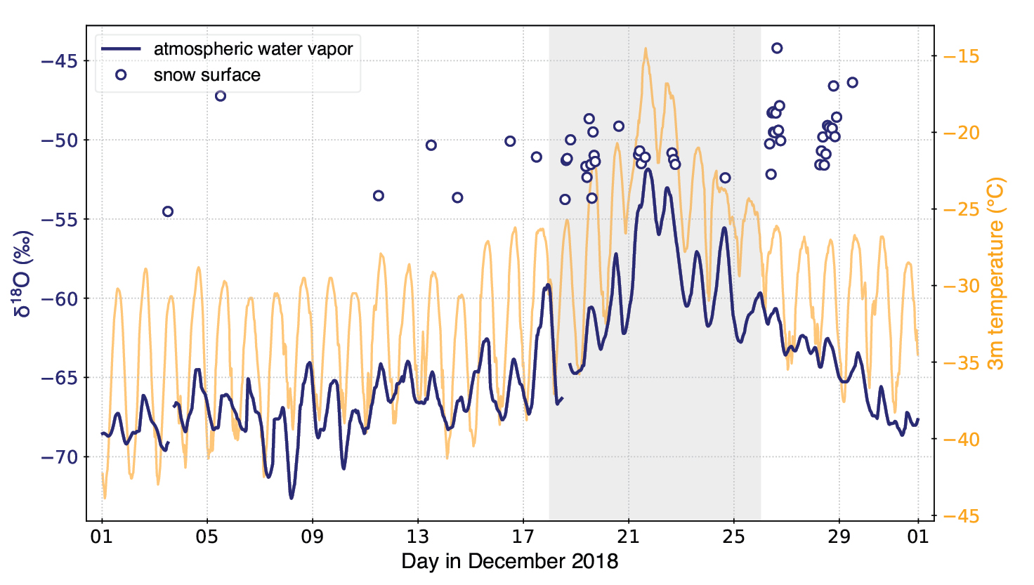 |
Figure 2: Observed isotopic composition of snow and atmospheric water vapor and local air temperatures at Dome C in December 2018. δ18O was measured using a PICARRO laser spectrometer (atmospheric water-vapor data in Leroy-Dos Santos et al. 2021) and air temperature was measured by a sensor installed at three meters above the ground (data in Genthon et al. 2021). The atmospheric river event is marked by the gray shading. |
Lastly, precipitation samples collected in the field over several years have permitted the establishment of a temporal relationship between the snowfall δ18O and the ambient temperature of 0.49‰/°C. It is significantly lower than the spatial slope of 0.8‰/°C obtained from various datasets of Antarctic snow, and traditionally used for temperature reconstructions (Masson-Delmotte et al. 2008; Stenni et al. 2016). This further highlights the importance of such measurements for the interpretation of δ18O records in ice cores.
Summary
While water-isotope records from ice cores can provide invaluable information on past climate variability, their quantitative interpretation in terms of temperature has been challenged by recent studies that revealed the impact of several processes at the surface of the ice sheet, modifying the isotopic composition of the snow after precipitation. Research is still ongoing to disentangle and quantify the impact of these different processes, which take place during the archiving of the snow, on the isotopic climate signal found in ice cores. For this reason, field measurements are performed, and provide some of the keys to understanding the dynamics of the water isotopes at the surface of the Antarctic Ice Sheet.
affiliations
1Geophysical Institute and Bjerknes Centre for Climate Research, University of Bergen, Norway
2Laboratoire des Sciences du Climat et de l’Environnement, Université Paris-Saclay, Gif-sur-Yvette, France
3Department of Environmental Sciences, Informatics and Statistics, Ca’ Foscari University of Venice, Italy
contact
Inès Ollivier: ines.ollivieruib.no
REFERENCES
Casado M et al. (2016) Atmos Chem Phys 16: 8521-8538
Casado M et al. (2018) The Cryosphere 12: 1745-1766
Casado M et al. (2021) Geophys Res Lett 48(17): e2021GL093382
Cauquoin A, Werner M (2021) J Adv Model Earth Syst 13(11): e2021MS002532
EPICA community members (2004) Nature 429: 623-628
Genthon C et al. (2016) Int J Climatol 36: 455-466
Genthon C et al. (2017) Atmos Chem Phys 17: 691-704
Genthon C et al. (2021) Earth Syst Sci Data 13: 5731-5746
Leroy-Dos Santos C et al. (2021) Atmos Meas Tech 14: 2907-2918
Libois Q et al. (2014) J Geophys Res Atmos 119: 11662-11681
Masson-Delmotte V et al. (2008) J Clim 21: 3359-3387
Steen-Larsen HC et al. (2014) Clim Past 10: 377-392
Stenni B et al. (2016) The Cryosphere 10: 2415-2428
Wahl S et al. (2021) Geophys Res Atmos 126(13): e2020JD034400
New modeling combined with radar observations show that North Patch, near Dome C, presents an exciting potential ice-core drilling location where ice up to 2 Myr old may exist with a detectable paleoclimatic signal.
Drilling for old ice in Antarctica
Ice cores offer scientists an invaluable record of the climate of the past. Whether we are studying the composition of the ancient atmosphere in air bubbles or analyzing water isotope ratios (δ18O and δD) to infer past temperatures, obtaining the oldest ice possible remains a challenge for ice-core research. Currently, the oldest continuous ice core comes from the European Project for Ice Coring in Antarctica (EPICA) at Dome C (EDC), which has given us a climate record from the past 800 kyr (Bazin et al. 2013). The International Partnerships in Ice Core Sciences (IPICS) community set the Oldest Ice challenge of extracting a continuous ice core which covers over 1 Myr (Fischer et al. 2013). An ice-core record of this length would allow us to directly measure past atmospheric greenhouse gas concentrations. It would also help us to understand the change in the periodicity of climate cycles, which occurred between 1.2–0.7 Myr BP, known as the Mid-Pleistocene Transition (Clark et al. 2006). Fischer et al. (2013) determined that a potential Oldest Ice site should have a low accumulation rate and a relatively thin ice sheet to avoid basal melting, and minimal horizontal ice flow, as basal sliding can cause distortion or even folding of the deepest, oldest ice (Dahl-Jensen et al. 2013).
The European Beyond EPICA consortium selected a site and began drilling in 2021 at a location known as Little Dome C (LDC) on the East Antarctic Plateau, where they hope to find ice up to 1.5 Myr old. The Australian Antarctic Division has also selected a site on LDC for their Million Year Ice Core (MYIC) project. In this article, we look at North Patch (Parrenin et al. 2017), an area approximately 10 km north of EDC. Our preliminary age modeling presents North Patch as an exciting prospect for a new Oldest Ice drill site with ice potentially up to 2 Myr old.
1D numerical age-depth model
Our model determines the age of ice, past accumulation rates and melt rate at a given location. It is a 1D model which means it only considers the vertical flow of ice and takes into account three parameters. The first parameter is the model’s best-fit ice-sheet thickness. From the difference between the best-fit ice thickness and the observed ice thickness, we can infer either a basal melt rate or a layer of stagnant ice (ice with no vertical flow). The second model parameter is the average past snow accumulation rate whose temporal variations can be inferred using the EDC ice-core record (Bazin et al. 2013). The accumulation rate corresponds to an annual snowfall which forms a layer on the surface of the ice sheet. Subsequent snowfall covers and compresses the snow below, slowly turning it into ice. As each layer is compressed further, it becomes thinner and moves deeper, as time goes by. The final parameter in the model accounts for this thinning process.
We provide the model with known age-depth constraints from observations made with radar surveys. We can use radar systems to send a signal deep into the ice sheet, and from the reflections we can detect the internal structure of the ice sheet. The radar images show internal reflection horizons. Since the ice at each horizon was formed from snow which fell at the same time, under the same conditions, the age of the ice along a given horizon is constant. By connecting these radar lines to the EDC age-depth profile, we can determine their ages. Taking into account the three model parameters mentioned above –mechanical ice thickness, average past accumulation rate, and the thinning parameter– the model fits the ages of these isochrones and the surface, and extrapolates down to the bedrock to give us a complete age profile along the radar line.
Modeling at North Patch
At North Patch, the sledge-borne DEep LOoking Radio Echo Sounder (DELORES) was used to collect radar data from 21 lines in a 5x5 km2 grid (Chung et al. 2023). From these data, 20 isochrones were dated by linking them to EDC with four radar lines (Fig. 1). The isochrones were then used to constrain a 1D numerical model.
The model is able to determine the age of ice at a given depth from the surface. The maximum age of the ice at a given location is either at the bedrock, or if the age density is equal to 20 kyr/m (20,000 annual layers per vertical meter). At this limit, paleoclimate reconstruction becomes impossible as obliquity cycles cannot be distinguished, at least using current experimental techniques (Fischer et al. 2013). Figure 1a shows that the maximum ice age predicted by the 1D model is generally between 2.2 and 1.9 Myr, around 500 kyr older than the expected age at the current Beyond EPICA drill site. The age density for 1.5 Myr-old ice at North Patch is generally between 9 and 11 kyr/m, which is twice as good as what we expect to find at Beyond EPICA (Chung et al. 2023) (Fig. 1b).
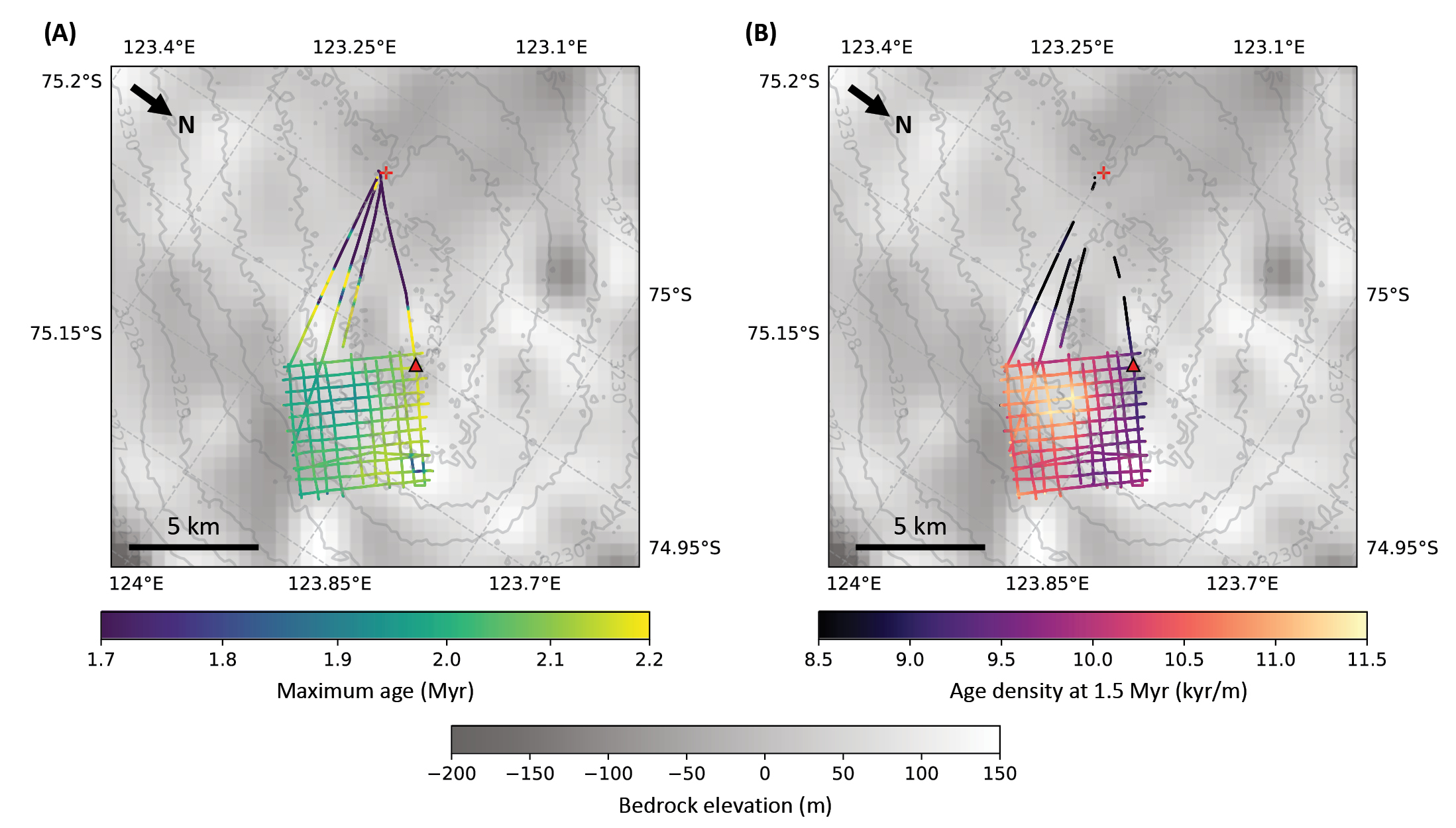 |
Figure 1: The model was run using 20 horizons traced in DELORES radar data at North Patch. The red cross marks EDC and the red triangle marks a promising North Patch site shown in Figure 2. (A) Modeled maximum age of ice at North Patch. (B) Modeled age density of 1.5 million-year-old-ice at North Patch. |
Modeling showed that there is very little, if any, basal melting at North Patch. There is also significantly less stagnant ice, which means that the climate record could be analyzed over the entire ice column. This results in thicker annual layers than at LDC, which would give us larger ice samples to analyze.
Potential North Patch drill site comparison
We chose a promising Oldest Ice location at North Patch and compared the age-depth relationship with that of the EDC and Beyond EPICA ice-core sites (Fig. 2).
The EDC ice core gave us a climate record (Fig. 2) which could be analyzed along almost the entire length, as the large ice thickness meant that age density was relatively low (Bazin et al. 2013). However, basal melting meant that the paleoclimatic record older than 800 kyr had been distorted, or completely destroyed (Tison et al. 2015). Modeling suggests that there is no basal melting at the Beyond EPICA drill site on LDC and there could be ice up to 1.5 Myr-old (Fig. 2). However, due to the thinner ice sheet, the oldest ice is likely to have very small annual layer thicknesses (one meter of ice covers over 20 kyr, Chung et al. 2023), so diffusion processes may make it difficult to interpret the paleoclimatic record. The modeling in Chung et al. (2023) shows that an ice core at North Patch could offer a middle ground (Fig. 2). This ice sheet is around 3200 m thick, resulting in lower age density, but there also appears to be little-to-no basal melting, leaving the oldest ice intact.
Outlook
The DELORES radar system is not the highest resolution available, therefore, it would be beneficial to apply newer radar systems to North Patch in order to confirm the findings in our study. The logistics of constructing a drill site at North Patch would be eased due to its proximity to the French-Italian Concordia station. Despite this, the age modeling suggests that the ice-core age-depth relationship at North Patch would be very different to those of EDC and Beyond EPICA (Fig. 2).
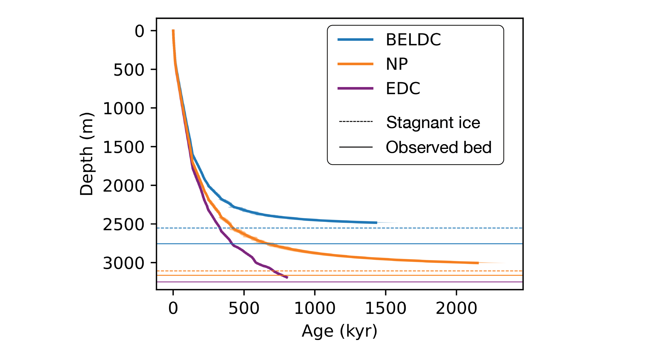 |
Figure 2: Age-depth profile of EDC (purple) determined experimentally (Bazin et al. 2013), modeled profiles for Beyond Epica LDC (BELDC) – the current ice-core drill site for Beyond EPICA (blue) project (Chung et al. 2023) - and for a promising North Patch site (orange). Dashed lines show the top of the stagnant ice layer, and solid lines show the bedrock depths observed in radar data in colors corresponding to each location. |
All that remains to be determined is who will choose to exploit this great opportunity to extract the (up to 2 Myr-old) Oldest Ice available at North Patch.
affiliationS
1Institute of Geosciences and the Environment, Université Grenoble Alpes, France
2British Antarctic Survey, Cambridge, UK
3Alfred Wegener Institute, Helmholtz Centre for Polar and Marine Research, Bremerhaven, Germany
4Department of Geosciences, Universität Bremen, Germany
contact
Ailsa Chung: ailsa.chunguniv-grenoble-alpes.fr
references
Bazin L et al. (2013) Clim Past 9: 1715-1731
Clark PU et al. (2006) Quat Sci Rev 25: 3150-3184
Dahl-Jensen D et al. (2013) Nature 49: 489-494
Fischer H et al. (2013) Clim Past 9: 2489-2505
An outstanding question of the Quaternary glacial cycles is the gradual emergence of a precession signal. Its absence in the Early Pleistocene may be explained by Northern Hemisphere ice sheets varying out-of-phase with a dynamic Antarctic ice sheet.
The Quaternary glacial cycles and Milankovitch’s theory
The Quaternary period (from ~2.6 Ma to present) is renowned for the cyclical growth and decay of large ice sheets in the Northern Hemisphere (NH). An important archive of this climate variability is the oxygen isotope ratio of benthic foraminifera (hereafter benthic δ18O) recovered from deep-sea sediment cores. Temporal variability in benthic δ18O serves as a proxy for changes in global ice-volume and deep-ocean temperatures. Lisiecki and Raymo (2005) compiled numerous records to produce a globally averaged “stack” of benthic δ18O for the last 5 Myr BP (LR04) with more positive values indicative of glacial conditions (Fig. 1a). Spectral analysis of this stack demonstrates that glacial cycles have a quasi-regular 100-kyr periodicity for the last ~0.8 Myr BP, together with smaller 23-kyr and 41-kyr cycles (Fig. 1b). Thereafter, shorter cycles begin to emerge with a regular 41-kyr period (Figs. 1c–d). The transition from the “41-kyr world” of the Early Pleistocene (from ~2.6 Ma to ~1.2 Ma) to the “100-kyr world” of the Late Pleistocene (from ~0.8 Ma to present-day) is referred to as the Mid-Pleistocene Transition (MPT).
Since the first δ18O measurements of marine sediment cores, the importance of changes in the Earth’s orbit around the Sun for pacing glacial cycles has been widely acknowledged. In particular, there are oscillations in the eccentricity of the Earth’s orbit with periods of 100-kyr and 400-kyr, the obliquity (tilt) of the Earth’s rotational axis with periods of 41-kyr, and the precession of the Earth’s rotational axis and orbital path with periods of 19- and 23-kyr. Variations in these three orbital parameters led to a redistribution of solar radiation received at the top of the atmosphere in space and time. Milankovitch (1941) hypothesized that summer insolation at the high northern latitudes was critical for the stability of ice sheets by controlling summer melting. Indeed, spectral analysis of deep-sea sediment and ice-core records support the importance of orbital cycles for Quaternary climate variability (Figs. 1b–d).
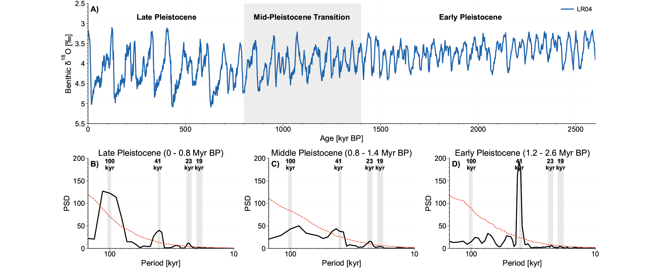 |
Figure 1: (A) The LR04 benthic δ18O stack from Lisiecki and Raymo (2005) and the power spectral density (PSD) of the (B) Late, (C) Middle and (D) Early Pleistocene using the multi-taper method from the Pyleoclim python package (Khider et al. 2022). Red lines denote 99% significance level. |
The Mid-Pleistocene Transition and precession cycles
On the other hand, Milankovitch’s theory cannot explain the MPT based on radiation changes alone, nor the ~100-kyr cycles of the Late Pleistocene. The MPT occurred with no major changes in the variations of Earth’s orbital parameters. The ~100-kyr cycles which followed the MPT coincide with variations in the Earth’s eccentricity, despite this orbital parameter having a negligible influence on summer-insolation intensity. Theories for the MPT are abundant. They include changes in the dynamics of NH ice sheets (Bintanja and van de Wal 2008) and changes in atmospheric CO2 concentrations (Raymo et al. 1988). For the 100-kyr glacial cycles of the Late Pleistocene, glacial terminations cluster into intervals of 80- and 120-kyr, and have been explained as a combination of two to three obliquity cycles (Huybers 2007).
Another ongoing question of the Quaternary is the absence of strong precession cycles in the Early Pleistocene. Climatic precession modulates the distance of the Earth relative to the Sun at the solstices and equinoxes, which leads to significant variations in summer-insolation intensity, as exemplified by insolation changes at 65ºN during the summer solstice (Figs. 2a–b). Indeed, the conspicuous absence of this precession signal (Fig. 1d) has been referred to as Milankovitch’s other unsolved mystery (Raymo and Nisancioglu 2003). Other studies reveal more significant precession variability in the Early Pleistocene (Liautaud et al. 2020), but also demonstrate a strengthening of precession across the Quaternary, as shown in Figures 1b–d. So, what causes the strengthening of these precession cycles?
Precession counterbalancing and integrated summer insolation
One process that diminishes the precession forcing is a counterbalancing that exists between summer-insolation intensity and the duration of the summer. When the Earth is closest to the Sun during the summer of either hemisphere, there is a prominent increase in insolation intensity. However, due to Kepler’s second law, the Earth has a higher orbital velocity when closer to the Sun, and subsequently the length of the summer season becomes shorter. Huybers (2006) demonstrates that the time-integral of the summer-insolation forcing above a critical threshold causes these two effects to largely cancel each other out, which can significantly reduce the precession variability (as shown in Figs. 2a–b). What then caused the precession signal to become stronger in the Late Pleistocene? Huybers and Tziperman (2008) suggest that a gradual cooling across the Quaternary would shorten the summer melt season and lessen this counterbalancing effect, together with a southward extension of the NH ice sheets into latitudes more sensitive to precession. However, there is the possibility of another contributing factor to the strengthening of precession cycles which lies in Antarctica.
Antarctica and the anti-phased hypothesis
Precession-driven changes in summer insolation are out-of-phase between the hemispheres. With this in mind, Raymo et al. (2006) propose that precession-driven variations of Antarctica and the NH ice sheets may have cancelled each other out in globally averaged proxies of ice volume. This concept can be illustrated by using a simple model of ice-volume change (Imbrie and Imbrie 1980) to simulate variations of both a Southern Hemisphere (SH) and NH ice sheet (Fig. 2c). The nondimensional model simulates the lagged response of each ice sheet to changes in local summer insolation and the output has been scaled to ±40 m of ice volume in the NH and up to ±20 m in the SH. We can see by progressively increasing the variability of the SH ice sheet that these hemispherically out-of-phase precession cycles increasingly interfere with each other, leaving behind a stronger 41-kyr obliquity signal in global ice volume (Fig. 2d). In this way, the notable absence of a precession signal in the Early Pleistocene could be explained by the cancellation of out-of-phase precession cycles between the SH ice sheet (i.e. Antarctica) and the NH ice sheets. Intrinsic to this hypothesis is the notion that the mass balance of Antarctica is driven by changes in local summer insolation, as proposed by Raymo et al. (2006) for the Early Pleistocene. What then caused the increase in precession variability recorded across the Pleistocene? A gradual cooling across the Quaternary would lead to the development of a marine-based Antarctica with virtually no surface melting, as observed today. Together with the gradual expansion of the NH ice sheets, this stabilisation of Antarctica would decrease the ratio between SH and NH ice-volume variations, enhancing the precession signal observed in global ice volume (as shown in Fig. 2d).
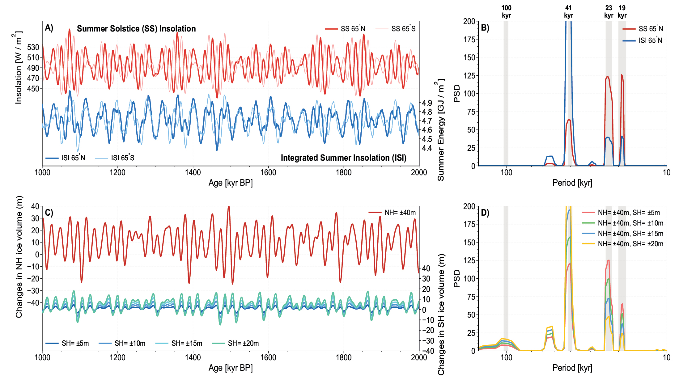 |
Figure 2: (A) Changes in summer solstice and integrated summer insolation for 65ºS and 65°N and (B) their respective PSD. (C) Modeled variations of a SH and NH ice sheet using a nondimensional ice-volume model (Imbrie and Imbrie 1980) which simulates their lagged response to summer solstice insolation at 65ºS and 65ºN. (D) The model output is scaled for ice-volume variations of up to ±20 m for the SH ice sheet and ±40 m for the NH ice sheet, to illustrate how precession-driven variations of the SH and NH ice sheet can cancel each other in the global record. Panels (C) and (D) replicate plots from Raymo et al. (2006). |
Outlook
Interestingly, a strengthening of precession cycles across the Quaternary, driven either by a reduction in the counterbalancing effect between summer-insolation intensity and duration and/or an increasing imbalance between NH and SH precession cycles, requires a cooling across the Quaternary. However, reconstructions of CO2 across the MPT have produced conflicting results (Hönisch et al. 2009; Yamamoto et al. 2022). On the other hand, the anti-phased hypothesis predicts that Antarctic temperatures should vary in-phase with local summer insolation in the Early Pleistocene, as has been suggested by ice cores recovered from the Allan Hills Blue Ice Area (Yan et al. 2022). Ultimately, the arrival of the Beyond EPICA Ice Core will prove important to test the anti-phased hypothesis by providing a high-resolution record of changes in CO2 and local Antarctic temperatures across the MPT.
affiliations
1Department of Earth Science, University of Bergen and the Bjerknes Centre for Climate Research, Norway
2Université Grenoble Alpes, CNRS, IRD, Grenoble-INP, IGE, France
3Institute for Marine and Atmospheric research Utrecht and the Department of Physical Geography, Utrecht University, The Netherlands
contact
Daniel F.J. Gunning: daniel.gunninguib.no
references
Bintanja R, van de Wal RSW (2008) Nature 454: 869-872
Hönisch B et al. (2009) Science 324: 1551-1554
Huybers P (2006) Science 313: 508-511
Huybers P (2007) Quat Sci Rev 26: 37-55
Huybers P, Tziperman E (2008) Paleoceanogr 23: PA1208
Imbrie J, Imbrie J (1980) Science 207: 943-953
Khider D et al. (2022) Paleoceanogr Paleoclim 37: e2022PA004509
Liautaud PR et al. (2020) Earth Sci Plan Lett 536: 116137
Lisiecki LE, Raymo ME (2005) Paleoceanogr 20: PA001071
Raymo ME et al. (1988) Geology 16: 649-653
Raymo ME et al. (2006) Science 313: 492-495
Raymo ME, Nisancioglu KH (2003) Paleoceanogr 18: 1011
 |
Ice cores are unique in that they are the only archives that enable direct measurement of gas composition of the past atmosphere. To date, the longest continuous ice-core record covers the last 800,000 years and was retrieved from the EPICA Dome C ice core (Jouzel et al. 2007). The next challenge is to understand the climatic transition from 41-kyr to 100-kyr glacial cycles which occurred between 1.2 to 0.7 Myr BP, known as the Mid-Pleistocene Transition (MPT) (Gunning et al. p. 58). The aim of the Beyond EPICA–Oldest Ice Core (BE-OIC) project is to drill an ice core as old as 1.5 Myr to obtain a continuous, high-resolution paleoclimatic record, including past greenhouse gas concentrations, which would cover the MPT. The BE-OIC project began in 2019 and drilling is scheduled to reach bedrock in 2026. The BE-OIC drill site (75.29ºS, 122.44ºE) on the East Antarctic Plateau was chosen for its low snow accumulation rate and topographic conditions, which are conducive to old ice (Chung et al. p. 60).
The oldest ice of the BE-OIC is characterized by very thin layers, which presents a major challenge to study. In preparation for the analysis and interpretation of the core, the DEEPICE Marie Sklodowska-Curie doctoral network was created to train the next generation of ice-core scientists. DEEPICE consists of 15 PhD students working at 10 institutions across Europe with 11 non-academic partner organizations.
This issue presents a selection of current research topics related to the DEEPICE PhD projects. Firstly, water isotope (δ18O and δD) signals in ice cores are commonly interpreted as a temperature proxy, but they can be altered by surface processes (Ollivier et al. p. 62). Another challenge is to develop new techniques to measure and interpret these signals in the extremely thin layers of the deepest, oldest ice, which are discussed by Malegiannaki et al. (p. 64) and Shaw et al. (p. 66).
Impurities in ice can provide information about climatic changes. For example, mineral dust can tell us about atmospheric circulation changes and organic molecules can be used as tracers of past biospheres. Ongoing methodological developments enable the characterization of single dust particles (Lee et al. p. 68) and increase the number of detectable organic analytes (Notø p. 70). Laser ablation mass spectrometry shows that most impurities are located at grain boundaries between ice crystals (Larkman et al. p. 72). Moreno et al. (p. 74) explore the potential of large area scanning microscopy for the macro-scale analysis of the ice-crystal size.
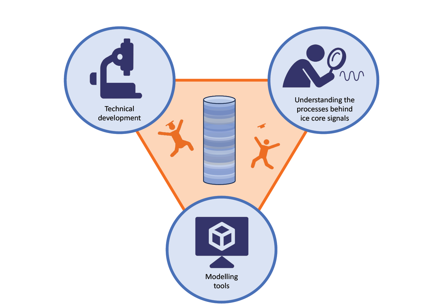 |
Figure 1: The three areas that the DEEPICE PhD students are working on to improve ice-core analysis and climate signal interpretation techniques for the BE-OIC project. |
The interpretation of climate data requires accurate dating, which becomes complicated for the deepest ice. This is why new dating methods using radionuclides (Kappelt et al. p. 76) and the gaseous O2/N2 ratio are under development (Harris Stuart et al. p. 78). The latter can also be used to reconstruct the atmospheric O2 content. Past atmospheric concentrations of nitrous oxide are difficult to reconstruct because this greenhouse gas is produced in the ice. Soussaintjean et al. (p. 80) investigate this process to isolate the atmospheric signal of nitrous oxide.
The analysis and interpretation of gases in ice cores also requires an understanding of how air bubbles transform into air hydrates, which are ice “cages” filled with gas molecules (Painer et al. p. 82). At greater depths, the ice close to the bedrock contains debris and elevated gas concentrations, which could provide novel insights into the history of the ice sheet (Ardoin p. 84).
The developments in ice-core science from the DEEPICE project will enable us to study the only archive that combines continuous high-resolution climate signals with a direct record of the past atmospheric gas composition. A better understanding of past climate will help constrain models of ice-sheet and climate evolution (Gao et al. p. 86). The BE-OIC ice-core data will complement existing paleoclimatic records and assist in unraveling the mystery of the MPT.
ACKNOWLEDGEMENTS
The articles of the DEEPICE special section of this magazine have received funding from the European Union’s Horizon 2020 research and innovation programme under the Marie Sklodowska-Curie grant agreement No 955750.
 |
The opinions expressed, and arguments employed herein, do not necessarily reflect the official views of the European Agency.
affiliationS
1Institute of Geosciences and the Environment, Université Grenoble Alpes, France
2Department of Geology, Lund University, Sweden
3Alfred Wegener Institute, Helmholtz Centre for Polar and Marine Research, Bremerhaven, Germany
4Department of Geosciences, Eberhard Karls University, Tübingen, Germany
5Climate and Environmental Physics, Physics Institute and Oeschger Centre for Climate Change Research, University of Bern, Switzerland
contact
Lison Soussaintjean: lison.soussaintjeanunibe.ch
references
Beyond EPICA–Oldest Ice Project
The PAGES Data Stewardship Scholarship program contributed to the development of an online database interface and a visualization tool of past sea level by the PALSEA working group.
The creation of reporting standards for sea-level proxies and the compilation of sea-level databases have been a central focus of the PALeo constraints on SEA level rise (PALSEA) working group (pastglobalchanges.org/palsea) since its inception (Düsterhus et al. 2016; Rovere and Dutton 2021). Over the last three years, these efforts came to fruition with two products. First, a global database of post-Last Glacial Maximum (LGM) sea-level index points was created within the Geographical variability of Holocene sea level (HOLSEA) project (Khan et al. 2019). Second, the creation of the World Atlas of Last Interglacial Shorelines (WALIS; Rovere et al. 2022) database, which includes sea-level proxies dating back to Marine Isotopic Stage (MIS) 5.
With the completion of these two databases, ideas started to arise concerning the feasibility of uniting them under a single interface and the availability of visualization and interfaces to allow for their exploration, and facilitate data query and download. With these ideas in mind, we submitted a proposal for a Data Stewardship Scholarship to PAGES. The proposal had two primary goals. The first was to implement the Holocene sea-level data standard format (Khan et al. 2019) into the interface built for the WALIS database (available here: alerovere.github.io/WALIS), eventually duplicating the database done within the HOLSEA project into WALIS. The second goal was to provide a visualization interface for the WALIS data, taking inspiration from the one already proposed for the HOLSEA database (Drechsel et al. 2021).
The first result of our work was the implementation of the HOLSEA data template into the WALIS database structure, including the online database interface. This work is now complete. As a result, any user logging into the WALIS online data insertion interface will not only be able to insert MIS 5 data, but will also find a series of tabs dedicated to the insertion of standardized Holocene data, including tables for radiocarbon, U-series, archaeological, and other age attribution methods. The Holocene part of the WALIS interface is currently undergoing beta testing, but is fully functional. After this phase, we plan to release a non-beta version of the interface, populated with the post-LGM data already in the HOLSEA database.
 |
|
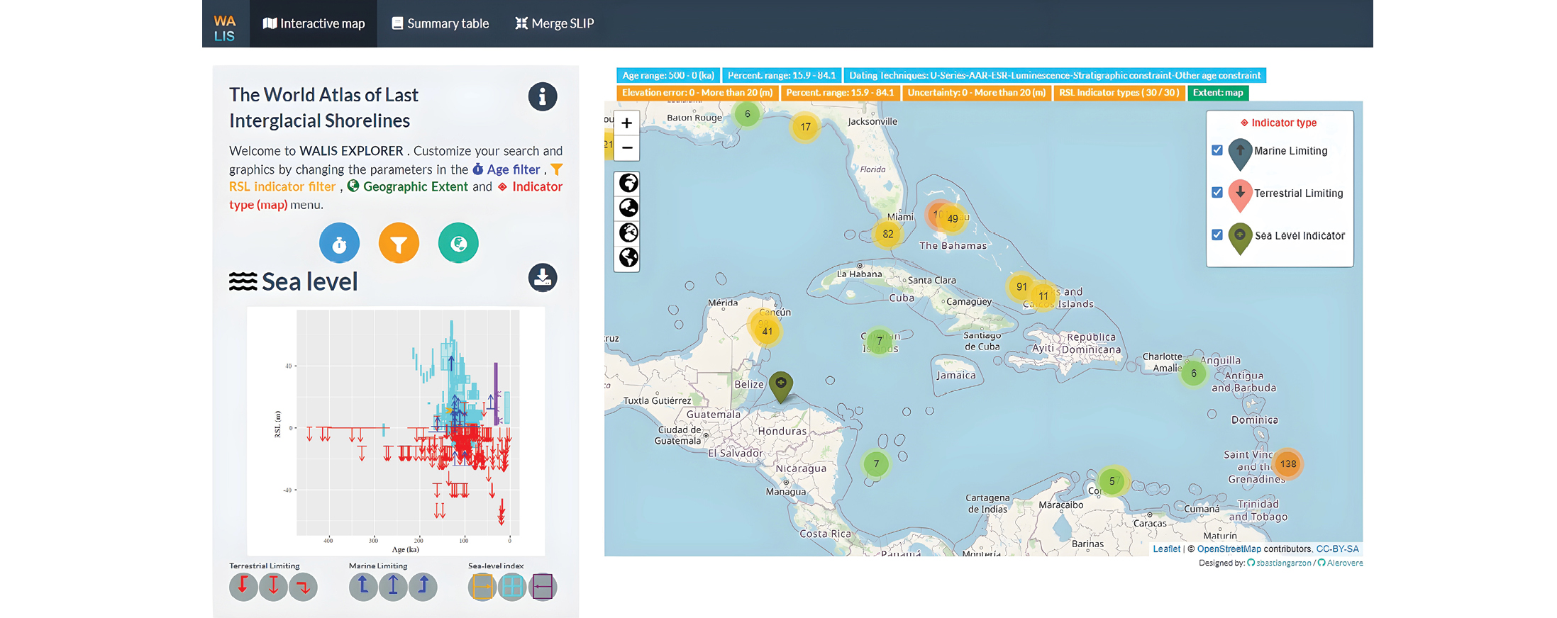
Figure 1: A screenshot of the WALIS Data Explorer application. |
The second achievement of our work was the creation of a platform to query and analyze the data already included in WALIS. This work was done through an R Shiny App querying a simplified version of the WALIS database (i.e. including only the essential fields related to indicator type, paleo sea level and dating information). The app is currently in its 2.0 version. The code to run the app offline is available from Garzón and Rovere (2022), and the app is also accessible online at this link: warmcoasts.shinyapps.io/WALIS_Visualization/. The application is divided into three pages, which the user can navigate. On the first page, it is possible to filter the data by geographic selection, age, elevation, or indicator type. On the second page, the app allows the previously selected data to be downloaded in .csv format. Finally, on the third page, the app allows further fine-tuning of the data query by excluding specific index points and calculating an age/sea-level probability density graph using a Monte Carlo approach.
The results briefly described above represent a fundamental stepping stone towards increasing the wide availability and usability of paleo sea-level data. Our data and code are fully open access. Bug reports and suggestions on how to improve the current products and forks to the GitHub repositories linked to the published code versions are also welcome.
ACKNOWLEDGEMENTS
Thanks to the European Research Council under the European Union’s Horizon 2020 research and innovation programme (grant agreement No. 802414) for funding the World Atlas of Last Interglacial Shorelines database WALIS (Rovere et al. 2022).
affiliations
1Department for Environmental Sciences, Informatics and Statistics, Ca’ Foscari University of Venice, Italy2MARUM, Center for Marine Environmental Sciences, University of Bremen, Germany
3Laboratory of Geo-information Science and Remote
Sensing, Wageningen University & Research,
The Netherlands
4Environmental Law Institute, Washington DC, USA
5Department of Earth Science, The University of Hong Kong, Hong Kong
contact
Alessio Rovere: show mail address
references
Drechsel J et al. (2021) Quat Sci Rev 259: 106884
Düsterhus A et al. (2016) Clim Past 12: 911-921
Garzón S, Rovere A (2022) WALIS visualization interface. Zenodo
Khan NS et al. (2019) Quat Sci Rev 220: 359-371
Rovere A, Dutton A (2021) PAGES Mag 29: 18-20
Rovere A et al. (2022) WALIS - The World Atlas of Last Interglacial Shorelines (Version 1.0). Zenodo
The PAGES Data Stewardship Scholarship program allowed us to organize and archive multiple published peat-based paleoecological datasets, increasing their accesibility and visiblity via cross-platform linking.
For many years now, the C-PEAT working group (pastglobalchanges.org/c-peat) has made available hundreds of peatland-carbon datasets. So far, these datasets only include limited information, namely age-depth model and peat geochemical data (bulk density, carbon and nitrogen content, etc.). But there is a wealth of peat-based paleo-proxy data that remains sparse in public repositories. The PAGES Data Stewardship Scholarship has allowed us to build a framework to organize and archive our community’s peat-based paleoecological datasets. We are also integrating this dataset to the Neotoma database (neotomadb.org). The interest has been high among the peat community to see peat records further integrated to regional paleoclimate reconstructions, such as the 2k Network (pastglobalchanges.org/2k). Increasing the accessibility and visibility of peat-core paleo-proxy data should help to fulfill this goal. We hope we can convince paleoclimatologists working with lake sediments, speleothems, tree rings, ice cores, and other archives of peat's promise!
Peatland archives
Peatlands are arguably the very first recognized paleoclimate archives. In the 19th century, the alternating dark and light layers from European peat deposits were interpreted as indications of warmer/drier and wetter/cooler conditions, respectively (Blytt 1876). These records of past climate change, which were based on plant macrofossils and pollen assemblages, led to the development of the first deglacial paleoclimate sequence: the Blytt-Sernander classification (Blytt 1876; Sernander 1908). Today, with thousands of peat profiles described and analyzed from every continent, peat-based paleoclimate work remains an active field of research.
Despite this long history and the large number of published studies, peat-based paleorecords remain somewhat underutilized. They are also seldom combined with those from other terrestrial archives, such as lakes, trees, and ice. Here we contend that peatland archives can offer complementary insights in Holocene paleoclimatology due to: (1) their global distribution, including regions where other terrestrial archives are rare; (2) their temporal coverage and resolution, which can offer decadal-scale Holocene reconstructions; and (3) their capacity to record changes in temperature, moisture source, or other climate components.
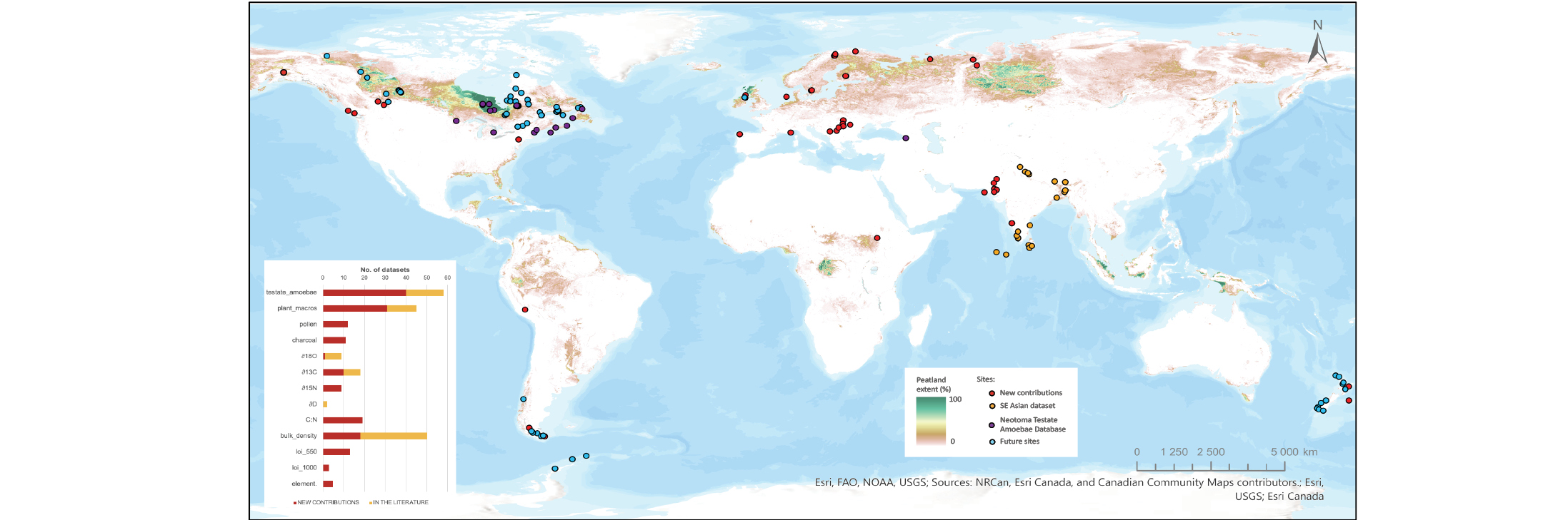 |
|
Figure 1: The Peatland Paleo Proxy Database as of 31 December 2022. It comprises 182 records from 101 cores. Orange = Neotoma Testate Amoebae Database; red = new proxy data contributions; blue = metadata only (for now). Modified from Melton et al. (2021). |
Data aggregation and formatting
Over the past two years, C-PEAT Data Steward Nicole Sanderson has gathered as many peat-based paleoecological datasets as possible. She led a number of "peat proxy happy hour" sessions to engage with data owners and facilitate data transfer. She trained a couple of undergraduate researchers (Kendahl Hejl and Daniel Maraldo) in data formatting and quality control. She became a Neotoma data steward and has been actively discussing the Peatland dataset with Neotoma leaders. These efforts have paid off: 182 chronologically constrained paleorecords from 101 cores have recently been processed by our team (Fig. 1). Those cores are globally distributed, though most of them are located in the Northern Hemisphere. The dataset includes chronologically constrained testate amoebae, plant macrofossil, and geochemical records, as well as novel proxies such as biomarkers and stable isotopes (Fig. 1). Prior to our work, Neotoma only contained 18 peat-based paleorecords. The newly formatted records are being integrated on Neotoma and should be available sometime this year.
Current and future plans
The Peatland Paleo Proxy Database will be available for community use on Neotoma, and we aim to continue to expand its contents in order to improve process-based models. This new C-PEAT database will be used to assess ecosystem responses to past environmental drivers, including recovery from past abrupt changes in water table depth and temperature, as well as building carbon trajectories. We also aim to integrate the peat-based paleorecords with other terrestrial records (e.g. lake sediments, tree rings) in regional paleoclimate reconstructions. Our team is preparing a manuscript that describes the proxies included in the dataset and the methods used to format, synthesize, and analyze the paleo peatland records. Ultimately, we aim to link this dataset through LiPD (lipd.net).
ACKNOWLEDGEMENTS
We would like to thank Kendahl Hejl and Daniel Maraldo for their help building the database; Socorro Dominguez Vidana and Simon Goring for their technical support through Neotoma; the C-PEAT community for sharing their datasets and knowledge.
affiliations
1Department of Geography, Texas A&M University, College Station, USA2Department of Geography, University of Quebec in Montreal, Canada
3Department of Geography, University of Exeter, UK
contact
Julie Loisel: juloiselhotmail.com
references