PAGES Magazine articles
Ice cores provide a record of atmospheric particles that could have affected past climate. Single-particle inductively coupled plasma time-of-flight mass spectrometry can measure size distributions, number concentrations, and elemental chemical composition of many thousands of individual insoluble nanoparticles and microparticles.
Particles in Earth’s atmosphere and climate
Atmospheric particles include sulfates, nitrates, black/organic carbon, sea salt, and mineral or other water-insoluble particles with diverse natural and anthropogenic sources (e.g. volcanic eruptions, desert dust, biomass burning, fossil-fuel combustion, sea spray). Compared to other climate forcings like carbon dioxide (CO2) and methane, atmospheric particles are irregularly distributed in the atmosphere, reflecting diverse sources, short lifetimes, and complex atmospheric transport conditions (Raes et al. 2000).
The chemical (e.g. mineralogy/elemental composition) and physical (e.g. size, solubility, density) properties of individual mineral atmospheric particles affect climate directly through absorption and scattering of solar radiation, and indirectly through changes in cloud and ice formation and structure (Haywood and Boucher 2000). Bioavailable iron-bearing particles can fertilize the ocean, creating algal blooms, thus, reducing the global CO2 concentration (Martin 1990). Particles with diameters <2.5 µm (“fine particulates”) containing toxic metals have negative impacts on human health (Shiraiwa et al. 2017).
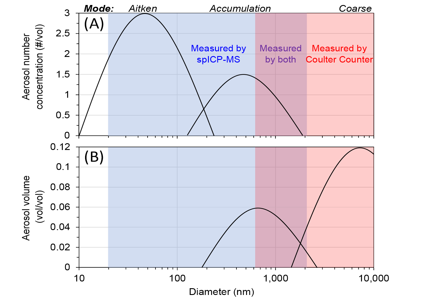
Most particles in the atmosphere and entrapped in ice cores (by number concentration) are classified within the Aitken mode size range (10 to 100 nm, nanoparticles), with a smaller but significant number within the accumulation mode size range (100 to 1000 nm, fine microparticles) (Seinfeld and Pandis 2006; see conceptual model particle size distributions in Fig. 1). However, particles within the Aitken mode contribute very little to the total mass (and volume) of particles, while most of the total mass (and volume) is in coarser particles. Glaciers are excellent archives of the Earth’s climate over hundreds of thousands of years, including deposited insoluble mineral atmospheric nanoparticles and microparticles. The physical and chemical characteristics of particles are indicative of the past atmosphere and can offer insight into how the Earth’s climate changed over time. Measuring particles entrapped in remote Antarctic ice can also provide a benchmark of comparison to the modern, anthropogenically affected atmosphere.
Here, we first discuss analytical techniques traditionally used to measure the particles entrapped in glacial ice cores. While useful, these methods cannot measure the elemental chemical composition of thousands of individual nanoparticles and fine microparticles. We then highlight single-particle inductively coupled plasma time-of-flight mass spectrometry (spICP-TOFMS) as a tool for measuring hundreds of thousands of individual mineral nanoparticles and microparticles.
Traditional techniques used to measure mineral atmospheric particles entrapped in glacial ice
Several analytical techniques, including Coulter Counter and Abakus, bulk analysis by inductively coupled plasma-sector field-mass spectrometry (ICP-SFMS), and transmission or scanning electron microscopy (TEM or SEM) with energy dispersive X-ray spectrometry (EDXS), are used to measure atmospheric particles in melted glacial ice.
Coulter Counters and Abakus are widely used to measure size distributions and number concentrations of accumulation and coarse mode insoluble particles larger than 500 nm (Fig. 1; Delmonte et al. 2002; Folden Simonsen et al. 2018) independent of the elemental-chemical composition of particles.
|
|
Figure 1: Theoretical lognormal size distributions of aerosol particles measured by spICP-MS displayed as (A) a function of number concentration and (B) volume/mass. Figure adapted from Seinfeld and Pandis 2006. |
Bulk analysis by ICP-SFMS determines average elemental concentrations in an acidified sample (McConnell et al. 2018; Uglietti et al. 2014). It is impossible to differentiate between contributions from chemically digested insoluble mineral particles, water-soluble particles, and dissolved ions in the sample. Bulk analysis cannot measure particle-number concentrations, size distributions, or individual particle compositions. Measuring low-abundance trace elements (e.g. Ir, Pt) is challenging and requires ultra-clean techniques in order to avoid contamination (Gabrielli et al. 2004).
SEM/TEM-EDXS determines the shape, size, and elemental chemical composition/mineralogy of individual particles. SEM/TEM-EDXS is a time-consuming technique which requires locating and scanning each individual particle. The time required to measure a statistically significant population (i.e. thousands or hundreds of thousands) of particles in a sample is prohibitively long. A limited number of studies have used TEM/SEM-EDXS to measure mineral nanoparticles and microparticles, with most focusing on common particles containing elements present at major or minor abundances in the Earth’s crust (Ellis et al. 2015).
Techniques to measure elemental composition and size of thousands of individual particles
Single particle mass spectrometry (SPMS) has been used since the 1990s to measure particles in the modern atmosphere in real-time (Noble and Prather 2000). In the only reported use of SPMS to measure particles in ice cores (Osman et al. 2017), long sampling times (>1 hour) and more than 100 mL of liquid sample were required, which can be a limitation in analyzing ice cores with small sample volume. Furthermore, SPMS typically does not quantify the amount of each element in a particle. Instead, the amount of each element is reported as a percentage of the total ion current detected.
Single-particle inductively coupled plasma-mass spectrometry (spICP-MS) is becoming widely used to measure engineered nanoparticles in the environment, biological samples, and food (Montaño et al. 2016). The particle suspension is nebulized and introduced into the ICP ion source. Unlike bulk ICP-MS which measures the average concentration of elements over a few seconds, spICP-MS measures the ion signal with a time resolution as short as 10 µs. While spICP-MS using a quadrupole or sector field MS can only measure one element per particle, spICP-TOFMS measures a complete elemental mass spectrum (up to 70 elements excluding O, H, N, F, and the noble gases) every 30 µs. Each particle produces a discrete burst of signal ~500 µs long (“particle event”); instrument software identifies mass spectra due to a particle event. The relationship between ion-signal intensity and the mass of each detected element is calibrated using solutions so that the amount (femtograms -fg- =10-15 grams) of each detected element can be quantitated. From the amounts of each detected element, the percentage of each element in the particle can be estimated. There was only one previous publication (Erhardt et al. 2019) that used spICP-TOFMS to measure particles in an ice core to our knowledge.
Measuring insoluble mineral particles by spICP-TOFMS
spICP-TOFMS is uniquely capable of quickly (in ~30 minutes) measuring the estimated mass equivalent size distribution, number concentration, and elemental chemical composition of more than 100,000 individual insoluble mineral nanoparticles and microparticles using only one milliliter of melted ice.
The mass-equivalent particle diameter is estimated for each particle using the total mass (in femtograms) of all detected element(s) and an estimated density (i.e. average crustal density, 2.7 g cm-3). The shape of the particle cannot be determined by spICP-TOFMS. spICP-TOFMS can detect particles as small as ~20 nm (that are too small to be measured by a Coulter Counter; Fig. 1).
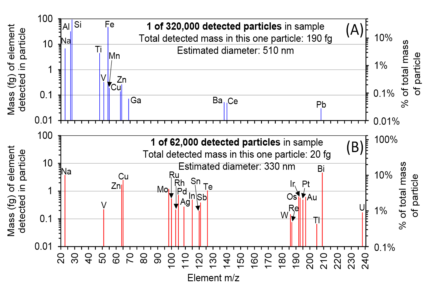
Figure 2 shows examples of mass spectra produced from two individual insoluble-mineral particles detected in Taylor Glacier ice samples by spICP-TOFMS. The top spectrum is from a common particle composed mainly of elements (e.g. Na, Al, Si, Fe, Zn, etc.) at major or minor concentrations in the Earth’s crust (Fig. 2a). The bottom particle contains ultra-low amounts (<10 fg) of uncommon elements such as Os, Au, Pt, Ir, and Tl (Fig. 2b). It would be difficult to measure these particles by bulk ICP-MS because the signal each element produces would be a very small fraction of the background signal integrated over several seconds.
|
|
Figure 2: Amount (mass, femtograms -fg-) of each element detected in an individual particle from (A) 17 kyr BP and (B) 11 kyr BP Taylor Glacier samples. 560,000 particles/mL were detected in the 17 kyr BP sample. 110,000 particles/mL were detected in the 11 kyr BP sample (m/z=mass/charge ratio of ion detected by mass spectrometer; used to identify each element from a characteristic isotope). |
Potential minerals and mineral groups can be inferred for each particle by comparing the ratio of the amounts of detected elements to known mineral elemental ratios. Common minerals (e.g. quartz, ilmenite, kaolinite) can be differentiated from particles with unusual compositions that would be undetectable by bulk ICP-SFMS, or challenging to find by SEM/TEM-EDXS. These particles can act as markers of very rare environmental events (i.e. micrometeorites; volcanic tephra from eruptions).
Conclusions and perspectives
Glacial ice cores contain crucial information about the size, number concentration, and elemental chemical composition of hundreds of thousands of insoluble mineral particles over Earth’s climatic and environmental history that were unmeasurable using conventional techniques. Measuring additional ice-core samples from the glacial–interglacial transition by spICP-TOFMS will give us a better understanding of the impact of mineral particles on past climate, and answer questions about how particle mineralogy, size, and number concentration changed over the glacial–interglacial timescale.
affiliationS
1Trace Element Research Laboratory, School of Earth Sciences, The Ohio State University, Columbus, USA
2Department of Chemistry and Biochemistry, The Ohio State University, Columbus, USA
3Byrd Polar and Climate Research Center, The Ohio State University, Columbus, USA
4Honeybee Robotics, Altadena, USA
contact
John Olesik: Olesik.2@osu.edu
references
Delmonte B et al. (2002) Clim Dyn 18: 647-660
Ellis A et al. (2015) Atmospheric Meas Tech 8: 3959-3969
Erhardt T et al. (2019) Environ Sci Technol 53: 13275-13283
Folden Simonsen M et al. (2018) Clim Past 14: 601-608
Gabrielli P et al. (2004) J Anal At Spectrom 19: 831-837
Haywood J, Boucher O (2000) Rev Geophys 38: 513-543
Martin JH (1990) Paleoceanography 5: 1-13
McConnell JR et al. (2018) Proc Natl Acad Sci 115: 5726-5731
Montaño MD et al. (2016) Anal Bioanal Chem 408: 5053-5074
Noble CA, Prather KA (2000) Mass Spectrom Rev 19: 248-274
Osman M et al. (2017) Atmospheric Meas Tech 10: 4459-4477
Raes F et al. (2000) Atmos Environ 34: 4215-4240
Shiraiwa M et al. (2017) Environ Sci Technol 51: 13545-13567
 |
This special issue highlights recent advances in ice-core paleoclimatology led by early-career researchers (ECRs) and reflects the efforts of the Ice Core Young Scientists (ICYS; pastglobalchanges.org/icys) workshop in October 2022 in Crans-Montana, Switzerland (pastglobalchanges.org/calendar/26967). These articles are dedicated to promoting ECR research at the frontiers of ice-core science, and they recognize the recent surge of development in novel ice-core proxies, ice-core dating, and modeling techniques over the last decade. This endeavor is divided into areas at the heart of our field today: interpretation of ice-core proxies such as impurities, water isotopes, and gases; paleo-chronological constraints; and data integration with models to reconstruct paleoclimate scenarios.
The first set of articles feature novel environmental proxies based on ice-core impurities, with a focus on analytical techniques and applications. Increasing observations of climate-relevant aerosols, and assessing their impact on the climate system, is a pressing need, particularly over the Southern Ocean where the unique and poorly observed aerosol properties limit the ability of global climate models to correctly simulate the radiative budget. Novel analytical techniques show great promise for characterizing the size, shape, and composition of ice-core impurities, providing crucial data for radiative transfer models. New insights into the radiative properties of aerosols are highlighted by Lomax-Vogt et al. (p. 90), who describe the recent advances in ice-core single-particle analysis, while Cremonesi and Ravasio (p. 92) review innovative ice-core optical techniques. Burgay (p. 94) explores the potential of non-target screening of ice-core organic compounds as a previously untapped archive of atmospheric composition.
Trapped bubbles of ancient air are one of the most unique components of the ice-core record (Fig.1a). These gases provide a direct window to study the atmosphere of the past. Among recent advances, Shackleton (p. 96) shows how noble gas ratios in the ice-core record are used to reconstruct past mean ocean temperatures. Interpretation of the gas record in older ice samples presents a challenge, especially where the stratigraphic order has been disturbed. Current efforts to extract paleoclimatic information are described by Yan (p. 98) who reviews the use of blue ice areas — where very old ice has flowed to the surface — to record changes in million-year-old greenhouse gases.
Water isotopes are a fundamental component of ice-core temperature reconstructions. Yet accurate calibration of this traditional paleothermometer is hindered by diffusion, precipitation intermittency, and wind redistribution processes, as Casado and Orsi discuss (p. 100). Davidge (p. 102) explains recent developments in clumped water-isotope analysis, which provides more detailed information about the path of a water parcel from evaporation at the source, to precipitation on the ice sheet.
Robust age models provide the foundation to interpret the relatively high-resolution paleoclimate records from ice cores (Fig. 1b). Bouchet et al. (p. 104) showcase how Antarctic glaciological models for older ice are tuned using dating constraints from orbital parameters, the geomagnetic field, and volcanic eruptions. Fang et al. (p. 106) describe how radiocarbon in shallow Alpine ice cores can be used to resolve detailed climate records over the Holocene. Soteres et al. (p. 108) describe surface exposure dating of 10Be, a cosmogenic nuclide, on Patagonian glaciers to date millennial-scale climate shifts that resemble signals seen in both Greenland and Antarctic ice cores.
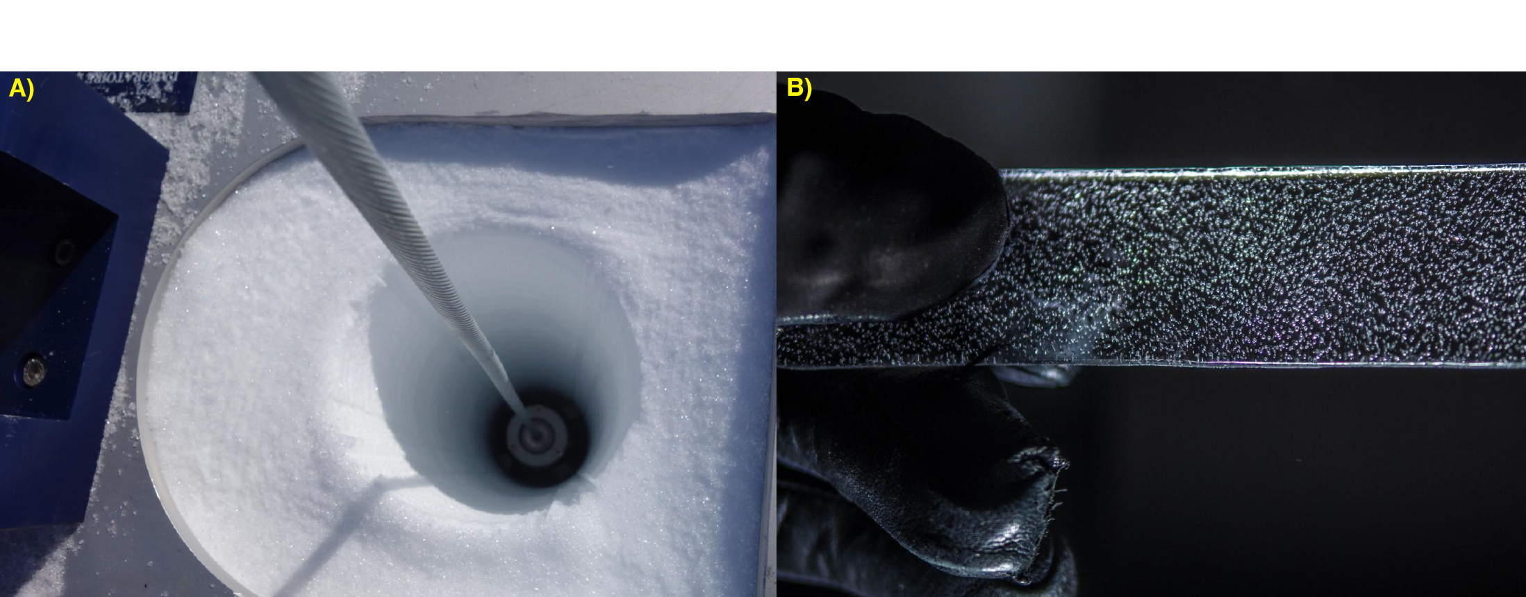 |
Figure 1: (A) Looking back through time down an ice-core borehole. Photo credit: LSCE, GLACCIOS. (B) Visible air bubbles in an ice core recovered from Talos Dome. Photo credits: A. Grisart and J-W. Yang. |
Integrating ice-core data with models is crucial to reliably forecast anthropogenic global warming. Slattery and Sime (p. 110) assess the effectiveness of ice-core data in statistical tools to pinpoint the timing of abrupt changes from Greenland glacial records.
affiliationS
1Antarctic Research Centre, Victoria University of Wellington, New Zealand
2Physics of Ice Climate and Earth, Copenhagen University, Denmark
3College of Earth, Ocean, and Atmospheric Sciences, Oregon State University, Corvallis, USA
contact
V. Holly L. Winton: holly.winton@vuw.ac.nz
To refine moisture-source and site-temperature reconstructions inferred from measurements from ice cores, we must understand moisture provenance from which Antarctic precipitation originates. Here, we discuss our current understanding of Antarctic precipitation origins and some recent modeling developments.
Why study Antarctic precipitation?
Antarctic precipitation is crucial to many aspects of the climate system. Firstly, Antarctic snowfall influences sea level through freshwater storage and ice-dynamic discharge. For instance, increased Antarctic snowfall might have mitigated global mean sea-level rise by ~10 mm during the 20th century (Medley and Thomas 2018). Secondly, enhanced atmospheric heat transport associated with increased Antarctic precipitation could promote polar amplification (Hahn et al. 2021). In addition, deep ice cores drilled in Antarctica enable us to understand how the Antarctic and global climates varied over hundreds of thousands of years. Water isotope (δ18O and δD) measurements from these ice cores have been used to infer past surface climate changes (e.g. Jouzel et al. 2007). By obtaining information about evaporation conditions of the precipitation, such as relative humidity and wind speed, we can tackle some key uncertainties in the interpretation of these isotopic measurements from ice cores.
How do we investigate Antarctic precipitation and its origin?
Because of its importance, continental and regional variations in Antarctic precipitation have been studied from daily to inter-annual timescales for many decades. For example, daily snowfall has been measured using a wooden platform at EPICA Dome Concordia (Dome C) since 2006 (Schlosser et al. 2016). Similarly, individual site measurements, which use snow stakes across Antarctica, allow observations of precipitation changes across the continent (Lenaerts et al. 2019). Invaluable larger-scale satellite measurements of precipitation over Antarctica have been available since the launch of CloudSat in 2006, though these measurements remain subject to calibration uncertainties (Palerme et al. 2014).
Complementary to observations, atmospheric general circulation models, which are sometimes run using data assimilation techniques, have provided precipitation and other relevant climate data for Antarctica. The European Centre for Medium-Range Weather Forecasts (ECMWF) combined numerous observations and a weather forecast model to produce the ECMWF Reanalysis v5 (ERA5, Hersbach et al. 2020). Based on the ERA5 dataset (1979–2022), average precipitation over the Antarctic Ice Sheet is ~175 mm/yr, and it decreases from coastal regions towards the Antarctic interior (Fig. 1a). Using multiple model simulations, Frieler et al. (2015) quantified the impact of a thermodynamic factor, i.e. the higher water holding capacity of a warmer atmosphere, on Antarctic precipitation. They found that, at the continental scale, Antarctic accumulation increases with temperature at a rate of ~5 %/K.
Combining ice-core data and reanalyses, Medley and Thomas (2018) investigated the Southern Annular Mode (SAM), which is the primary mode of atmospheric circulation variability in the southern mid-to-high latitudes. They found that SAM exerts regionally different controls over precipitation across Antarctica through modified moisture fluxes. Using a regional climate model, Turner et al. (2019) found that extreme precipitation events (EPE) contribute significantly to the amount and variability of Antarctic precipitation (Fig. 1b). It appeals for the study of dynamic drivers of EPE to project its future changes and impacts on Antarctic climate.
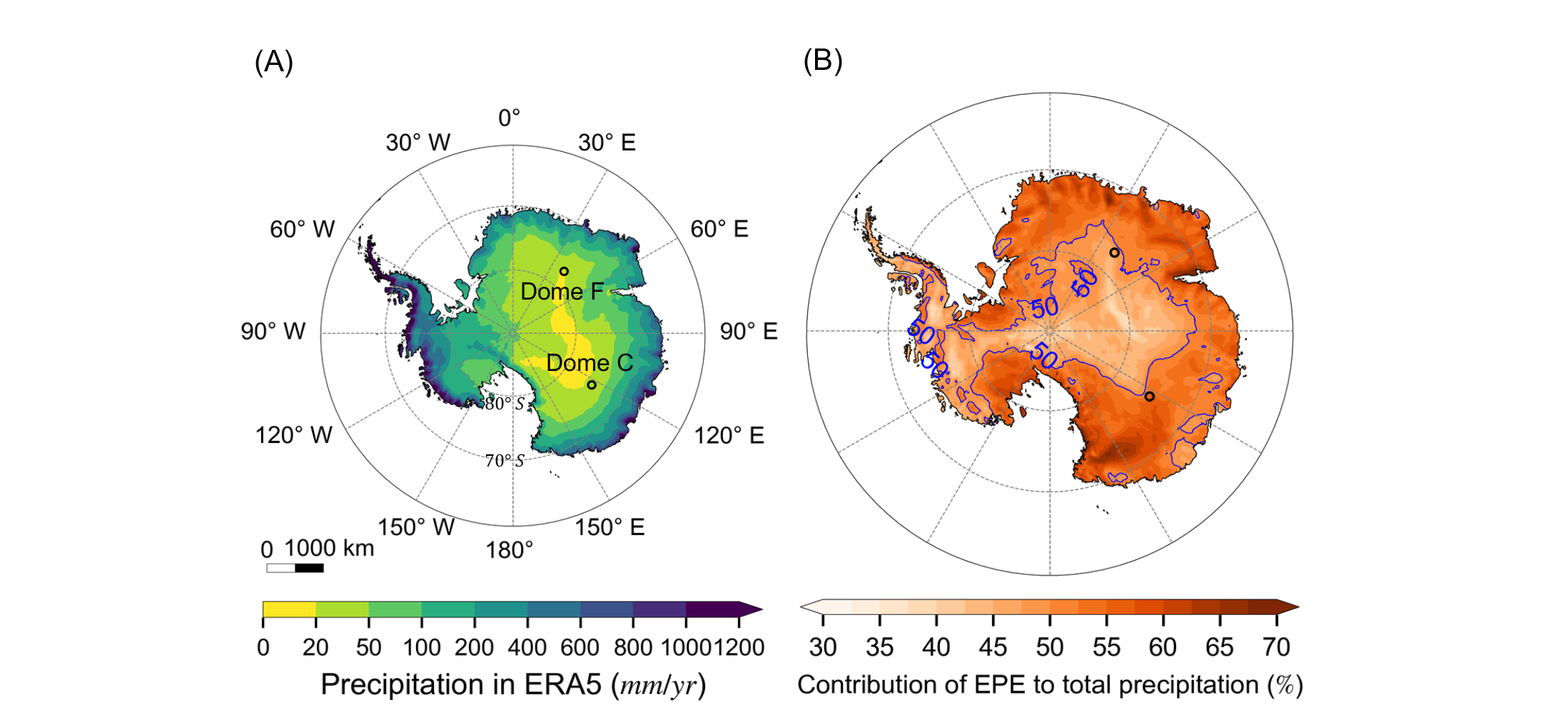 |
Figure 1: (A) Annual mean precipitation over Antarctica from the ERA5 reanalysis (1979–2022, Hersbach et al. 2020). (B) Contribution of extreme precipitation events (EPE) to total precipitation amount in the ERA5. Here EPE is defined as the top 10% heavy precipitation days following Turner et al. (2019). To help visual interpretation, blue lines show contours of 50% EPE contribution. |
Alongside these thermodynamic and dynamic controls, it is valuable to understand how the evaporative sources, and changes in these source properties, impact Antarctic precipitation. Water sources of Antarctic precipitation have thus been investigated using three different techniques.
Firstly, water isotope fractionation models can be applied to infer source temperature during evaporation processes based on deuterium excess data in Antarctic surface snow (Stenni et al. 2010). The deuterium excess is defined as the difference between the abundance of deuterium and 18O in water isotopes: d = δD – 8δ18O. This method relies on multiple assumptions, such as idealized moisture transport trajectories. Secondly, Lagrangian trajectory diagnostics can attribute moisture sources by identifying humidity changes along the transport of air parcels (Sodemann and Stohl 2009). However, even using 20-day backward trajectories instead of five-day trajectories as commonly used, moisture sources can be identified for only ~90% of total precipitation. Thirdly, atmospheric general circulation models simulate the global water cycle and are, thus, suitable for moisture-source attribution. A technique called "water tracing" in atmospheric models tracks moisture evaporated from prescribed regions until it precipitates. Traditionally, the globe is divided into multiple complementary regions, and then the contribution of each region to total precipitation at any location can be quantified. While the traditional approach has some downsides, such as being computationally expensive, recent progress in modeling developments has helped alleviate these issues, as discussed below.
Modeling advances in identifying moisture sources
Fiorella et al. (2021) developed a new and improved method for using water tracers in atmospheric models. This new method involves complex mathematical transformations throughout the water cycle, in addition to traditional water tracing. These new tracers allow for more precise inferences of environmental conditions during evaporation, transport, and condensation, making it possible to infer mass-weighted mean evaporation surface temperature and other parameters. This new approach is also much less computationally expensive.
Following on from this, we further developed and implemented this water-tracing approach in the state-of-the-art atmospheric model ECHAM6. We are also implementing the same water-tracing diagnostics in the Hadley Centre Global Environment Model version 3 (HadGEM3). Our water tracers provide abundant new information on moisture-source locations and evaporation-related properties of precipitation across Antarctica.
Figure 2 shows monthly precipitation and its evaporative source conditions at Dome C and Dome Fuji (Dome F). We find that annual mean oceanic-sourced precipitation has a source latitude of 37.6°S at Dome C and 35.1°S at Dome F (Fig. 2b). The source latitude reaches the most northern locations during December and January at both sites, and the most southern locations between March and May. Source sea-surface temperature (SST) of annual mean oceanic-source precipitation is approximately 14.7°C at Dome C and 16.1°C at Dome F (Fig. 2d). Note that annual mean oceanic-source precipitation is from more equatorward (by 2.5° in latitude) and warmer (by 1.4°C) waters at Dome F than at Dome C. Annual cycles of source SST are different from annual cycles of source latitude despite predominant meridional temperature gradients, mainly because of seasonal variations of SST at mid-latitudes. That is, at both sites, the source SST of monthly precipitation peaks in Austral summer (December to February) and is at its minimum in Austral winter (July to September). Although both sites receive moisture primarily from the west, the moisture source is located much further west for Dome F (~60°) than for Dome C (~10°).
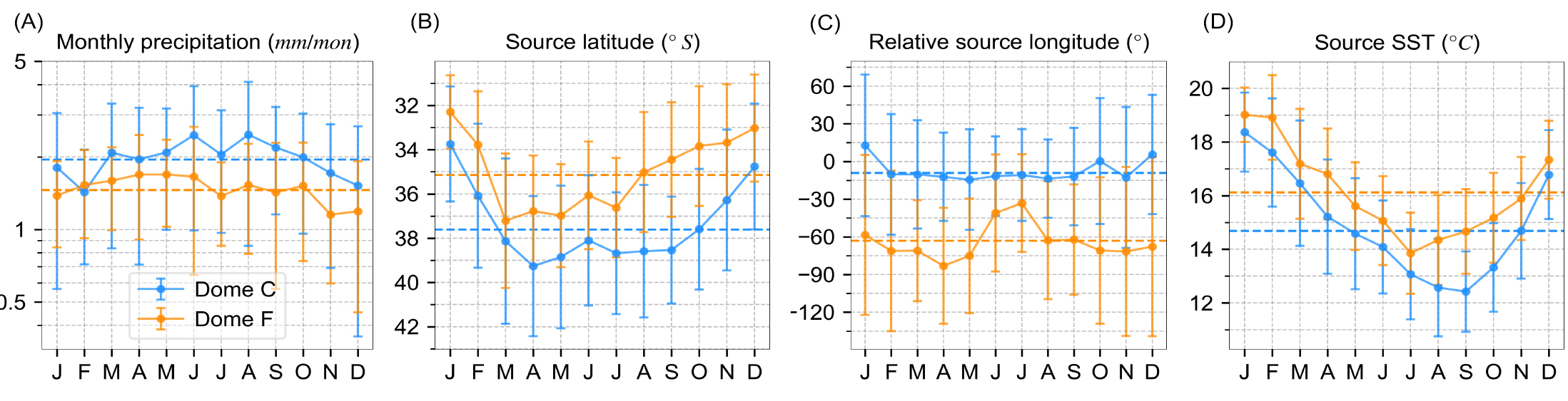 |
Figure 2: (A) Monthly mean precipitation at Dome C and Dome F. Panels show the (B) source latitude, (C) relative source longitude, and (D) source SST of monthly mean precipitation which originates from the open ocean. Data are from a preindustrial simulation using the atmospheric model ECHAM6. Moisture source information of precipitation at Dome C and Dome F is derived from our water-tracing diagnostics implemented in ECHAM6. Horizontal dashed lines represent annual mean values. |
Based on our moisture-source diagnostics, EPE derives its moisture from more northern regions by 3.0° and 3.7° than the rest of precipitation at Dome C and Dome F, respectively. The different moisture sources reflect distinct dynamic controls, which might imprint on water-isotope records.
Our current research aims to apply the water tracers to the study of paleoclimate. Indeed, measured water isotopes from Antarctic ice cores and the derived parameter deuterium excess have been interpreted for evaporation-source and precipitation-site temperature, based on simple water-isotope models (Landais et al. 2021). However, it is very challenging to quantify with atmospheric models the uncertainties associated with this method due to a lack of moisture-source information. Thanks to our new quantitative information on moisture sources, we will be able to refine uncertainty estimates attached to ice-core-based past temperature reconstructions from ice cores. In particular, future research will apply these new modeling tools to constrain local surface-temperature reconstructions from the ice core currently drilled at Little Dome C in the framework of the Beyond EPICA Oldest Ice Core project.
affiliationS
1Ice Dynamics and Paleoclimate, British Antarctic Survey, Cambridge, UK
2Department of Earth Sciences, University of Cambridge, UK
3Alfred Wegener Institute, Helmholtz Centre for Polar and Marine Research, Bremerhaven, Germany
4Institute of Environmental Geosciences, University of Grenoble Alpes, France
contact
Qinggang Gao: qino@bas.ac.uk
references
Fiorella RP et al. (2021) J Adv Model Earth Syst 13: e2021MS002648
Frieler K et al. (2015) Nat Clim Chang 5: 348-352
Hahn LC et al. (2021) Front Earth Sci 9: 725
Hersbach H et al. (2020) Qua J Roy Met Soc 146: 1999-2049
Jouzel J et al. (2007) Science 317: 793-796
Landais A et al. (2021) Nat Geosci 14: 918-923
Lenaerts JTM et al. (2019) Rev Geophys 57: 376-420
Medley B, Thomas ER (2018) Nat Clim Chang 9: 34-39
Palerme C et al. (2014) Cryo 8: 1577-1587
Schlosser E et al. (2016) Atmos Chem Phys 16: 4757-4770
Sodemann H, Stohl A (2009) Geophys Res Lett 36: L22803
Debris-rich basal ice layer of an ice sheet are shaped by processes at the bedrock which alter the paleoclimatic signal preserved in the ice. Basal layers offer insights on past ice-sheet dynamics and environmental conditions that emerged during ice-free conditions.
Greenland basal layers
Ice cores are a valuable source of information on past climate change because they provide insights into past atmospheric composition and temperature through the analysis of entrapped air and ice properties. In the Greenland Ice Sheet (GrIS) (Fig. 1a), the ice layers are well-defined and arranged in stratigraphic order down to a depth of a few hundred meters above the bedrock. Currently, the oldest continuous paleoclimatic record from the GrIS dates back to approximately 123,000 years ago (Landais et al. 2006). Below this depth, the ice becomes folded but still preserves some of the original paleoclimatic signal (Dahl-Jensen et al. 2013). However, even though basal ice may be less ideal for paleoclimatic research, the deepest part of the ice sheets still hold significant potential for preserving important paleoclimatic information. This is particularly true since silty ice dating back as far as 1 Myr has been retrieved from the deepest sections of the GrIS (Bender et al. 2010; Willerslev et al. 2007; Yau et al. 2016).
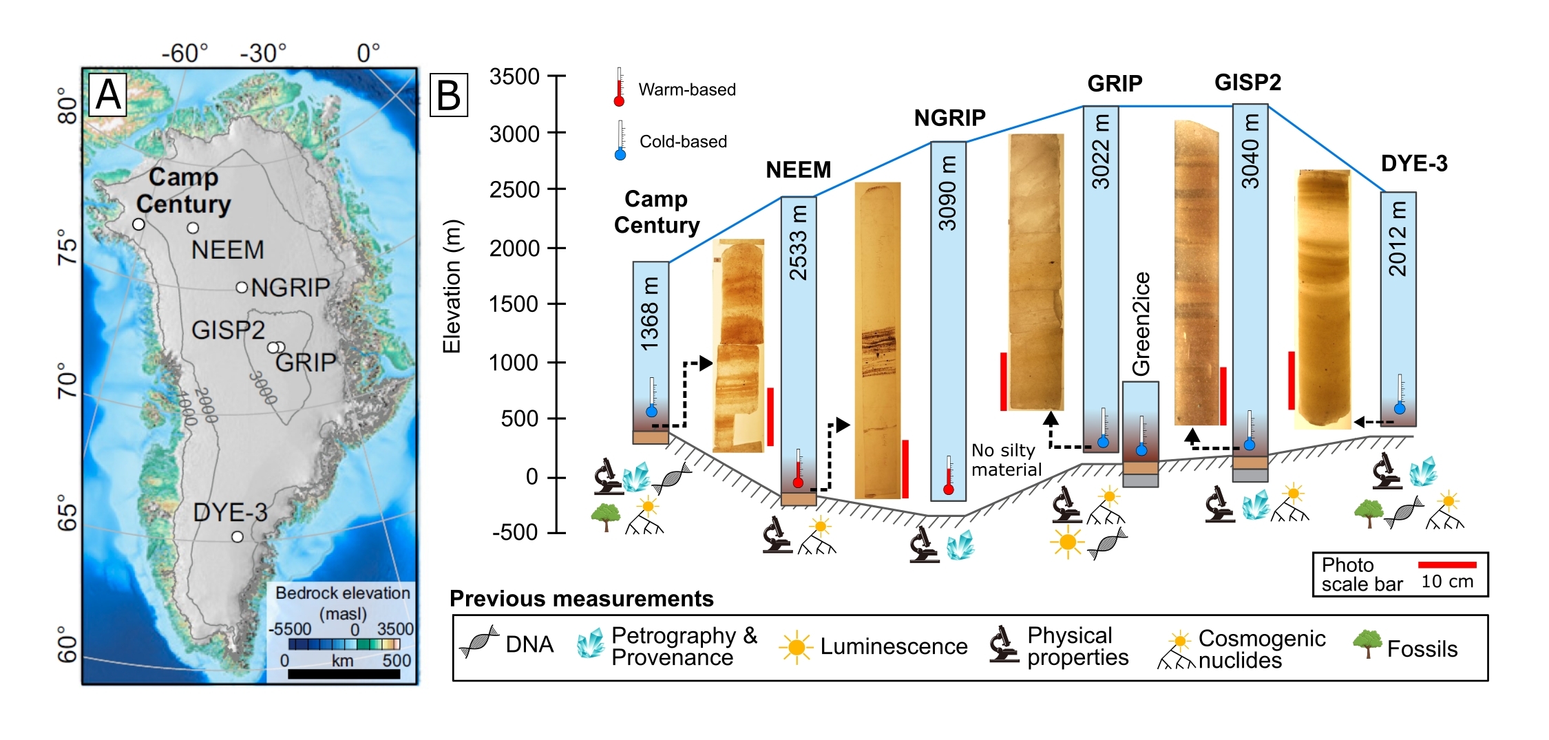 |
Figure 1: Synthesis of the studied ice cores from Greenland. (A) Ice-core locations and ice-surface elevation contours. (B) Ice-core thickness above the bedrock elevation (gray line), basal material thickness (exaggerated) and pictures of silty layers. Ice and gas chemistry were measured for all the ice cores. Modified from Christ et al. (2021). |
The basal ice can be divided into two categories: the so-called silty ice is made up of basal layers which contain debris incorporated from the bedrock (Fig. 1b), contrary to the basal clean ice that is already stratigraphically disturbed, but free of debris (sometimes referred to as “deep ice”). The gases (Fig. 2a) and water-isotopes measurements (Fig. 2b) from silty ice near the bottom of the ice sheet raises concerns about the preservation of paleoclimatic records (Fig. 2; Bender et al. 2010; Souchez et al. 2006; Verbeke et al. 2002).
Alteration of the paleoclimatic signal in basal ice?
The basal ice layers in the GrIS have unique properties that distinguish them from the overlying meteoric ice layers (derived from snow precipitation), including differences in ice texture, debris content, and gas composition (Bender et al. 2010; Goossens et al. 2016; Souchez et al. 2006; Tison et al. 2015). These layers exhibit heterogeneity at different scales, potentially involving a complex history of successive episodes of dynamic instability, melting and refreezing (Goossens et al. 2016), in situ biogeochemical processes, and diffusion from the sediments below.
The basal ice layers exhibit low gas concentrations, between 2 to 80% (Fig. 2a) of a typical meteoric ice concentration (Goossens et al. 2016; Tison et al. 2015). This is due to various processes such as gas rejection during melting/refreezing processes and pressure-expulsion of gas into subglacial cavities at lower local ambient pressures, e.g. downstream from bedrock obstacles.
However, a large accumulation of greenhouse gases in the silty ice are reported (up to 12% and 0.6% of CO2 and CH4, respectively), associated with a decrease in the O2/N2 ratio down to anoxic conditions (Fig. 2a; Herron et al. 1979; Souchez et al. 2006; Verbeke et al. 2002). This distribution cannot be solely explained by physical processes and requires mediation of microbial activity to account for it, either in the underlying sediments, in the ice itself, or in the soils prior to ice-sheet build up (Herron et al. 1979; Souchez et al. 2006; Verbeke et al. 2002). As the silty ice is at the interface between two contrasted environments (meteoric ice vs. underlying sediments/bedrock), its trapped gas signature may result from the mixing of two endmembers (Souchez et al. 2006). Mechanical ice mixing between a meteoric endmember and a locally derived endmember may explain both the incorporation of debris and changes in gas chemistry, superimposed on diffusion processes generated by potential gradients between contrasting endmember properties (water isotopes, impurities, and gas concentrations). However, the locally derived component must have been affected by microbial processes, resulting in a depletion of O2 (Souchez et al. 2006) and an accumulation of CO2 and CH4. This microbial signature may originate from a pre-existing marshy environment (Tison et al. 1998), which was eventually covered by the GrIS and trapped within the ice, or from the ecosystem prevailing in the subglacial environments.
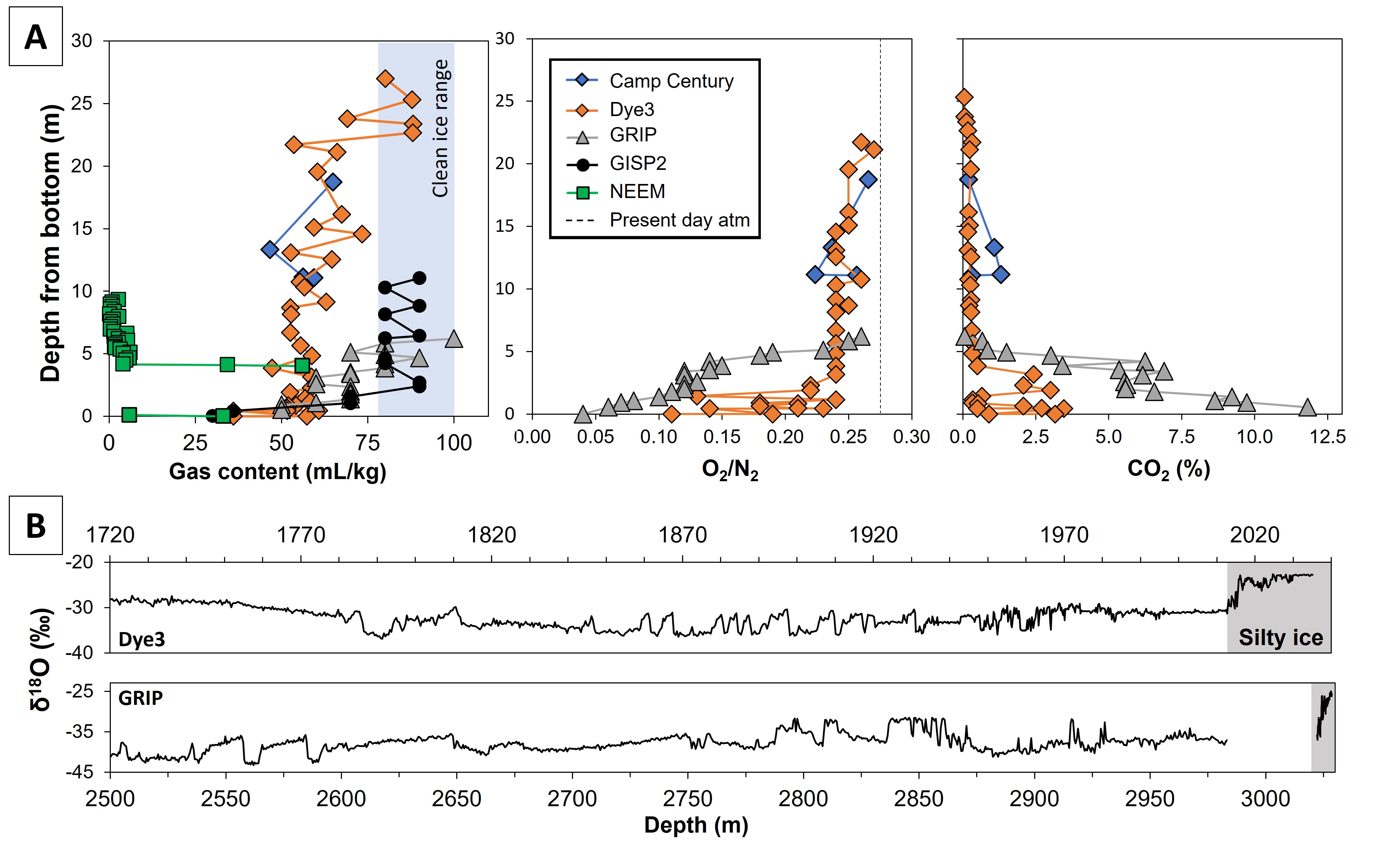 |
Figure 2: (A) Chemical proxies indicating variations between clean ice containing an atmospheric paleoclimatic signal and the silty layers of the Greenland Ice Sheet. (B) Ice δ18O record for the deepest section of Dye3 and GRIP. Data from Bender et al. (2010), Goossens et al. (2016), Herron et al. (1979), Souchez et al. (2006), Verbeke et al. (2002), and Yau et al. (2016). |
Stable water isotopes (δ18Oice and δDice) serve as useful tools for identifying stratigraphic discontinuities in basal ice layers, as they provide a clear paleoclimatic signal, being a proxy of air temperature in both Greenland and Antarctic ice-core records (Dahl-Jensen et al. 2013). Melting and refreezing processes can affect the relationship between δ18Oice and δDice (Souchez and Jouzel 1984), a process that could happen close to the bedrock. Therefore, stable water isotopes can shed light on the processes that affected basal ice layers during and after their formation. Another interesting feature observed in some silty ice layers in the GrIS is that their δ18Oice and δDice values are higher than those found in the overlying meteoric ice (Fig. 2b). This suggests that these layers may be the remnants of an earlier stage of the ice sheet’s growth, possibly from a time when the snow deposition occurred at a lower altitude (Souchez et al. 2006).
Unexplored paleoclimatic information in silty ice
Apart from traditional paleoclimatic proxies, the silty layers of the GrIS are becoming recognized as a valuable source of information on past ice-sheet dynamics. In addition, fossil remains, organic matter, and ancient biomolecules found in these layers provide insights into the types of ecosystems and environmental conditions that existed during periods of ice-free conditions (Fig. 1b). Recent research has demonstrated the potential of these layers to shed light on such key topics (Christ et al. 2021; Willerslev et al. 2007).
Analyses of mineral grains incorporated into the silty ice add constraints on the past waxing and waning (i.e. advance and retreat) of the GrIS. In situ-produced cosmogenic isotopes and the luminescence signal are two complementary methods constraining the past exposure and burial histories of under-ice sediments. The luminescence signal is indeed reset when the sediment is exposed to light. Under the ice cap, it rises because of the radioactive background of the geological environment. Thus, this luminescence signal can be used to date the last burial of the sediments during the last glacial advance. Alternatively, in situ-produced cosmogenic nuclides accumulate in quartz during ice-free conditions and decrease in concentration over time due to radioactive decay under the ice sheet. By coupling both methods, it is thus possible to constrain both the date of the last glacial ice-sheet readvance and the duration of the previous deglaciation (Christ et al. 2021; Schaefer et al. 2016). Additional constraints are provided by directly dating the basal ice, using dating techniques such as the 40Ar accumulation/degassing rate (Bender et al. 2010; Yau et al. 2016) and 81Kr in entrapped air (Buizert et al. 2014).
The ecosystems that occupied Greenland prior to the ice-sheet build-up, and during ice-free intervals, are poorly known because much of the fossil evidence is hidden below the kilometer-thick ice sheet. Terrestrial plant macrofossils, ancient molecules (DNA and lipid biomarkers, including their carbon and hydrogen isotopic composition) hold promises to unravel prevailing climatic conditions during ice-free intervals (Willerslev et al. 2007).
Despite stratigraphic disturbance and metamorphism effects, the basal layers of the GrIS, therefore, offer a unique opportunity to extend our knowledge about the history of the ice sheet and its (in)stability in a changing climate. The European Research Council Green2Ice synergy project will investigate this opportunity in the years to come (shorturl.at/kDFLN).
affiliation
Laboratoire de Glaciologie, Université Libre de Bruxelles, Belgium
contact
Lisa Ardoin: lisa.ardoin@ulb.be
references
Bender ML et al. (2010) Earth Planet Sci Lett 299: 466-473
Buizert C et al. (2014) Proc Natl Acad Sci 111: 6876-6881
Christ A et al. (2021) Proc Natl Acad Sci 118: e2021442118
Dahl-Jensen D et al. (2013) Nature 493: 489-494
Goossens T et al. (2016) The Cryosphere 10: 553-567
Herron S et al. (1979) J Glaciol 23: 193-207
Landais A et al. (2006) Clim Dyn 26: 273-284
Schaefer J et al. (2016) Nature 540: 252-255
Souchez R, Jouzel J (1984) J Glaciol 30: 369-372
Souchez R et al. (2006) Geophys Res Lett 33: 24
Tison JL et al. (1998) J Geophys Res Atmos 103: 18885-18894
Tison JL et al. (2015) The Cryosphere 9: 1633-1648
Verbeke V et al. (2002) Ann Glaciol 35: 231-236
Ancient air bubbles trapped inside polar ice sheets transform into clathrate hydrates at a certain depth. Not only do they contain the gas molecules used for paleoclimatic reconstructions, but they also serve as a climate proxy themselves.
Clathrate hydrates are solid guest-host compounds, formed by small molecules (guests; e.g. N2, O2, CH4 or CO2) trapped in a crystalline framework (host) of hydrogen-bonded water molecules (Chazallon and Kuhs 2002). In natural environments, clathrate hydrates occur in deep-sea sediments and permafrost (e.g. as methane hydrates). The first direct observations of clathrate hydrates of air (hereinafter, air hydrates) in polar ice were made in 1982 by Shoji and Langway (1982) in the Dye-3 ice core (Greenland) using an optical microscope. Subsequently, air hydrates have been found in all deep ice cores in Greenland and Antarctica (Uchida et al. 2014).
Air hydrate formation in polar ice
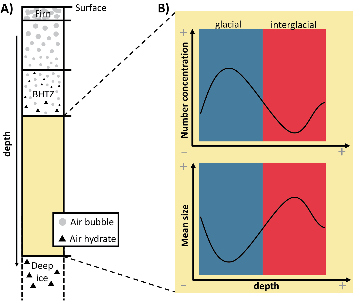
Air bubble inclusions in polar ice sheets are compressed with depth due to the increasing overburden pressure (e.g. Shoji and Langway 1982; Uchida et al. 2014). They transform into air hydrates below a certain depth, where the hydrostatic pressure enters the stability range of the clathrate hydrate at the in situ temperature (Uchida et al. 2011). The conversion occurs over a certain depth range, called the bubble-hydrate transition zone (BHTZ) (Fig. 1a), where bubbles and air hydrates coexist (Uchida et al. 2014). Its upper boundary is determined by the first appearance of a hydrate, the lower boundary by the last appearance of an air bubble.
|
|
Figure 1: (A) Schematic of an ice core and the occurrence of air bubbles and air hydrates at different depths. (B) Climate-dependent variations of the air-hydrate number concentration and mean size for the yellow depth range in A. |
For air-hydrate crystallization in the BHTZ, their (heterogeneous) nucleation is considered to be the rate-limiting step (Lipenkov 2000). Therefore, the starting depth and extent of the BHTZ varies (several hundred meters) for different ice-core sites in Greenland and Antarctica, owing to site-specific temperature and pressure conditions, as well as the occurrence of nucleation promoting or inhibiting factors (Uchida et al. 2014).
Given that air hydrates are formed from air bubbles, one could conclude that one bubble converts to one hydrate. However, a detailed investigation of the NGRIP (Kipfstuhl et al. 2001) and the Dome Fuji (Ohno et al. 2004) ice cores revealed that the number of total air inclusions (bubbles + hydrates) in the upper part of the BHTZ exceeds the air-bubble concentration above the transition zone.
Moreover, air hydrates in the transition zone show a wide variety of morphologies (Fig. 2a) and a non-uniform spatial distribution compared to air bubbles (Kipfstuhl et al. 2001; Lipenkov 2000; Ohno et al. 2004). The interpretation is that their formation is more complex (e.g. involving impurities; Ohno et al. 2004) than a simple one-to-one conversion and needs to be reinvestigated, including post-formation splintering and recrystallization mechanisms (Kipfstuhl et al. 2001).
Air hydrates and paleoclimate
Air hydrates are the source of at least two different types of information on paleoclimatic conditions. Firstly, they contain most of the air molecules in ice below the BHTZ and, as a result, provide a unique archive to reconstruct changes in past atmospheric gas compositions (Bereiter et al. 2015; Lipenkov 2000; Uchida et al. 2011, 2014). Secondly, some of the air hydrates’ geometrical characteristics (mean size and number concentration) correlate with past climatic changes (Lipenkov 2000). This has been shown for the Vostok and Dome Fuji ice core in Antarctica and the GRIP ice core in Greenland, where continuous records of air hydrates exist (Ohno et al. 2004).
In general, ice formed at glacial conditions is characterized by smaller air hydrates and a higher hydrate number concentration compared to ice formed at interglacial conditions (Fig. 1b) (Lipenkov 2000; Salamatin et al. 2003). This is essentially explained by the impact of past temperature and accumulation rate on the physical properties of the firn. For example, smaller ice-crystal grain sizes in colder firn lead to smaller air bubbles in ice. The original climate-dependent geometrical properties of air bubbles are then transferred to air hydrates (Lipenkov 2000).
After their formation, air hydrates are subject to an evolution with depth: the general trend of number concentration continuously decreases, coupled with an increase in the average size (Uchida et al. 2011). This phenomenon can be caused by a displacement of the hydrates and further fusion, and/or the diffusion of gas molecules and the subsequent growth of larger air-hydrate crystals at the expense of smaller hydrate crystals (a process called Ostwald ripening) (Salamatin et al. 2003; Uchida et al. 2011). This is especially pronounced in the deeper parts of the ice sheet, where it can even alter the original, climate-dependent variation of geometrical properties (Salamatin et al. 2003; Uchida et al. 2011). Increasing depth (and pressure), changes in temperature, and increasing age of the ice are the fundamental parameters behind this phenomenon (Uchida et al. 2011).
Material properties and analytical methods for air-hydrate studies
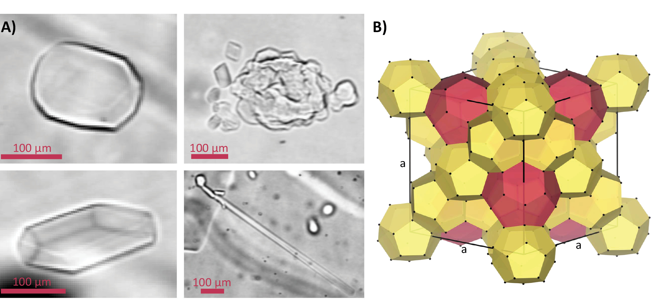
X-ray diffraction studies on single crystals of natural air hydrates in the Dye-3 ice core revealed the Stackelberg’s crystallographic structure II (sII) (Hondoh et al. 1990). It is one of the three main structures found for natural clathrate hydrates. The sII has a cubic unit cell which consists of 16 small cages and eight large cages formed by 136 water molecules (Fig. 2b) (Chazallon and Kuhs 2002). One or two guest molecules can be enclosed in each polyhedral cage, but not all cages need to be occupied. The nature of the guests, temperature, and pressure determine the crystal structure of the host framework and the degree of filling of the cages (Chazallon and Kuhs 2002).
|
|
Figure 2: (A) Microphotographs of different air-hydrate morphologies found in the bubble-hydrate transition zone of the EPICA-Dronning-Maud-Land ice core, taken with an optical light microscope (Kipfstuhl 2007). (B) Framework structure of the sII clathrate hydrate. The black cube (black line: a ~ 1.7 nm) represents the unit cell and the yellow and magenta polyhedra mark the small and large cages, respectively. The black dots at the polyhedra vertices mark the position of the oxygen atoms of water (dot size not to scale), the edges represent hydrogen bonds. This figure was created using VESTA 3 (Momma and Izumi 2011). |
Studying air hydrates in polar ice is challenging because they are thermodynamically unstable under temperature and pressure conditions in the field, or in the cold-laboratories, where samples are processed and inspected. However, the surrounding ice acts as a pressure cell to keep the hydrates metastable for a certain time, which depends on the ambient temperature conditions (Uchida et al. 1994). Consequently, for the long-term preservation of the record, appropriate storage conditions for the ice cores (≤ -50°C) are necessary (e.g. Bereiter et al. 2015; Uchida et al. 1994).
Optical light microscopy and cryo-Raman spectroscopy are the main non-destructive methods used to analyze air hydrates in polar ice. The microscope is the go-to tool for studying air-hydrate geometric properties. This investigation needs to be made as soon as possible after core retrieval, especially for the study of hydrates of the BHTZ (Kipfstuhl et al. 2001). Cryo-Raman spectroscopy enables the study of the main air-hydrate guest molecules (nitrogen and oxygen). In addition, this method can be used to analyze the various air-hydrate morphologies in 3D (Weikusat et al. 2015).
Outlook
There are still many open questions regarding the formation and evolution of air hydrates in polar ice. In the framework of Beyond EPICA and other Oldest Ice projects, a high analytical resolution and the development of new methodologies and climate proxies (e.g. dating via 81Kr decay or 40Ar/38Ar isotope ratio in entrapped air; Lipenkov et al. 2019) play a key role in analyzing highly thinned, and likely disturbed, deepest and oldest ice in Antarctica. A better understanding of the air-hydrate formation processes and their physicochemical properties is essential for using entrapped air in ice cores as a climate proxy. Certainly, this will improve the evaluation of measured gas concentrations (e.g. O2/N2 ratios or CO2; Bereiter et al. 2015). Equally important are the processes related to their evolution with depth (age) to further develop dating of very old (and disturbed) ice (Lipenkov et al. 2019).
affiliationS
1Alfred Wegener Institute, Helmholtz Centre for Polar and Marine Research, Bremerhaven, Germany
2Department of Geosciences, Eberhard Karls University, Tübingen, Germany
contact
Florian Painer: florian.painer@awi.de
references
Bereiter B et al. (2015) Geophys Res Lett 42: 542-549
Chazallon B, Kuhs WF (2002) J Chem Phys 117: 308-320
Hondoh T et al. (1990) J Incl Phenom Molec Recog 8: 17-24
Kipfstuhl S (2007) Thick-section images of the EPICA-Dronning-Maud-Land (EDML) ice core. PANGAEA
Kipfstuhl S et al. (2001) Geophys Res Lett 28: 591-594
Lipenkov VY et al. (2019) Geophys Res Abstracts 21: EGU2019-8505
Momma K, Izumi F (2011) J Appl Cryst 44: 1272-1276
Ohno H et al. (2004) Geophys Res Lett 31: 1-4
Salamatin AN et al. (2003) J Cryst Growth 257: 412-426
Shoji H, Langway CC (1982) Nature 298: 548-550
Uchida T et al. (1994) Mem Natl Inst Polar Res 49: 306-313
Uchida T et al. (2011) J Glaciol 57: 1017-1026
Uchida T et al. (2014) J Glaciol 60: 1111-1116
The production of N2O in glacial ice alters the record of past atmospheric concentrations of N2O in ice cores. Using isotope analyses of N2O would help understand the production processes and, thus, isolate the atmospheric signal.
Air bubbles trapped in ice cores represent the only direct paleo-atmospheric archive, and allow for, for example, the reconstruction of past greenhouse gas concentrations. But ice cores are not an inert medium; many chemical and physical processes take place in the ice. Under certain conditions, and for certain compounds, these processes can alter the signal stored in the enclosed air bubbles over time. The measured signals then no longer correspond exactly to the past composition of the atmosphere. Production of CO2 in Greenland ice cores and N2O in both Greenland and Antarctic ice cores are prominent examples for such an alteration of the atmospheric signal (Stauffer et al. 2003).
N2O: A growing climate threat
The study of N2O is important as it is a potent greenhouse gas that is also involved in the destruction of stratospheric ozone. The atmospheric concentration of N2O, with a global warming potential 273 times higher than CO2, has been increasing continuously over the past 150 years, reaching 332 ppb in 2019 (IPCC 2021). Currently, anthropogenic (mainly agricultural) sources contribute 43% of total N2O emissions, and natural sources from soils and oceans account for 57% (Tian et al. 2020). The main N2O sink is photochemical destruction in the stratosphere, and its preindustrial atmospheric lifetime is 123 years (Prather et al. 2015). Warmer climate seems to enhance natural N2O emissions, resulting in a positive feedback (Schilt et al. 2010a). This effect is difficult to predict because present and past N2O dynamics are poorly understood (Fischer et al. 2019). Reconstructed atmospheric N2O concentrations vary substantially on glacial-interglacial timescales (Flückiger et al. 2004; Schilt et al. 2010a). However, significant parts of the 800-kyr atmospheric record of N2O are missing due to in situ formation of N2O in glacial ice, rich in mineral dust (Fig. 1).
In situ production of N2O
Several observations indicate that the N2O concentrations measured in the ice are affected by a non-atmospheric source. For example, ice cores from different drilling sites show significantly different N2O values for given time periods (Schilt et al. 2010a, b). Considering the long atmospheric lifetime of N2O and, as a result, its geographically homogenous atmospheric concentration, this observation is inconsistent with only atmospheric N2O variations. The non-atmospheric source alters the N2O records exclusively during glacial periods, when the dust concentrations are high (Fig. 1). This indicates a production of N2O from compounds in, or attached to, aeolian dust deposited onto the ice sheet (Schilt et al. 2010a).
For most Antarctic ice cores, the dust-rich sections are almost entirely affected by in situ N2O production (Schilt et al. 2010a). Comparing different ice cores from Antarctica, the highest N2O concentrations are found in ice cores with the highest dust levels (Schilt et al. 2010b). In contrast, in situ N2O production in Greenland ice is not correlated with dust concentrations, and mainly occurs at the beginning and end of the Dansgaard–Oeschger events (Flückiger et al. 2004). Because these climatic transitions are associated with changes in chemical composition of the dust, N2O production is likely controlled by this factor.
Previous approaches
In situ N2O production represents a challenge for reconstructing the past atmospheric concentrations of N2O during glacial periods. To avoid misinterpretation in terms of past climatic variations and derived changes in marine and terrestrial sources, in situ production must be systematically detected.
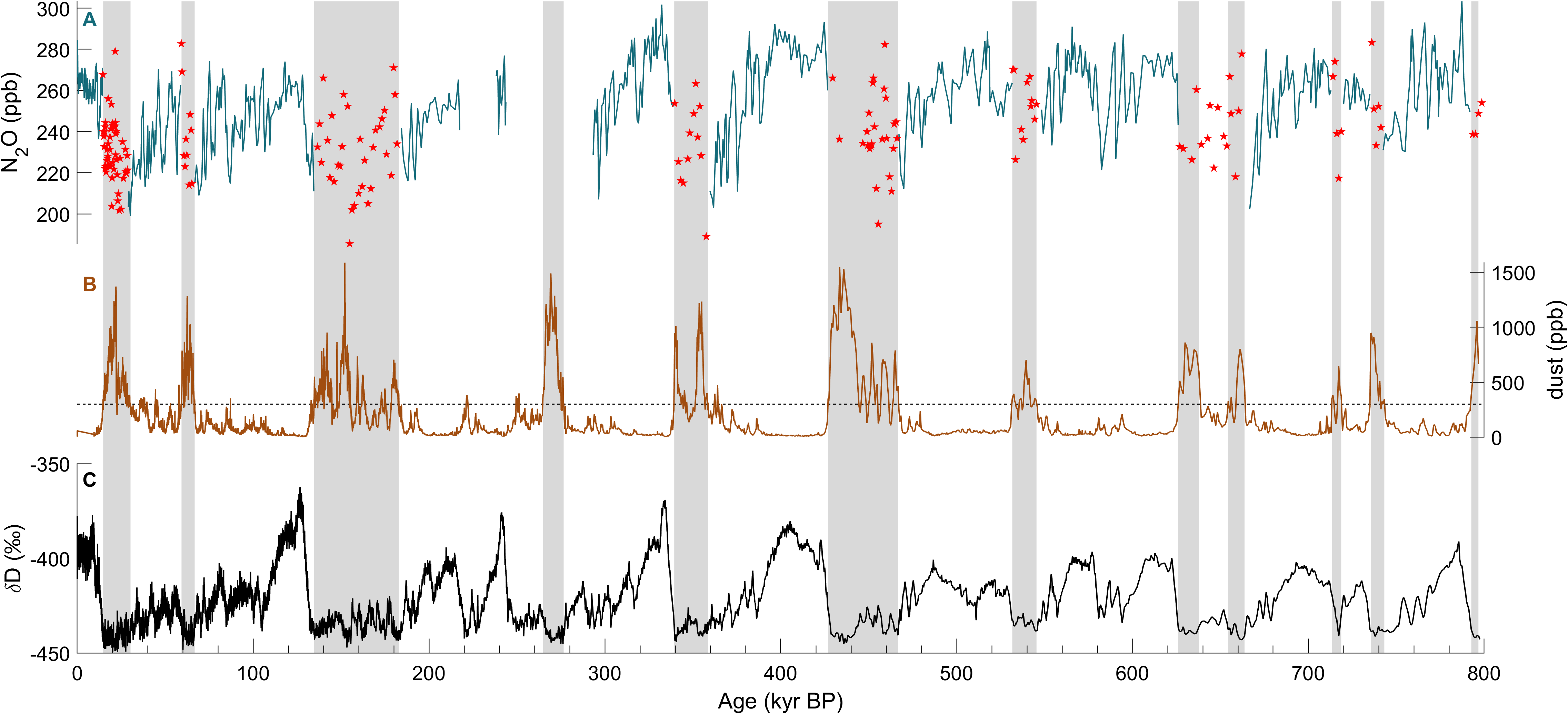
Flückiger et al. (2004) used a detection algorithm for Greenland ice that iteratively identifies N2O values exceeding a threshold of 8 ppb, which is about 3% of the typical glacial atmospheric concentrations, above a smoothing spline calculated through the whole dataset. However, this algorithm is only applicable to high-resolution datasets affected by erratic outliers, and is not valid for sharp rises in atmospheric concentration that could be mistaken for N2O outliers. The second approach, applied to lower-resolution records from Antarctic ice cores, identifies samples with a dust concentration above 300 ppb (Fig. 1; Spahni et al. 2005). This dust threshold is purely empirical and does not reflect the complexity of the N2O production. Indeed, if in situ N2O production in Antarctic ice is roughly proportional to the dust content, samples below this threshold may still be affected (e.g. at 640 kyr BP in Fig. 1). In summary, such detection algorithms help to improve the records, but are heuristic at best, and do not allow us to correct for the in situ contribution. For this, process understanding of the in situ formation is required.
|
|
Figure 1: (A) Measured N2O concentrations from the EDC ice core (Schilt et al. 2010a). Samples likely affected by in situ production are marked by red stars. (B) EDC dust concentration measured by laser scattering (Lambert et al. 2008). Gray-shaded areas mark sections with dust concentrations above the threshold of 300 ppb (dashed line). (C) EDC δD used as a temperature proxy (Landais and Stenni 2021). |
A new process-based quantification method
In the framework of the DEEPICE project, we seek to understand the processes responsible for N2O production. By identifying the chemical reaction at play, and the specific conditions necessary for its occurrence, we target three objectives: 1) to systematically detect the samples affected by in situ N2O to avoid misinterpretation of atmospheric N2O variations; 2) to quantify and predict the amount of in situ production in ice samples; and 3) to correct the N2O measurements to isolate the atmospheric N2O signal. Since isotope analysis is a powerful tool to trace sources of a compound, and previous work showed that the in situ fraction has an isotopic signature distinct from the atmospheric fraction (Fischer et al. 2019; Sowers 2001), our approach is based on the isotope analysis of N2O and impurities that may be precursors of the N2O in situ produced (Fig. 2).
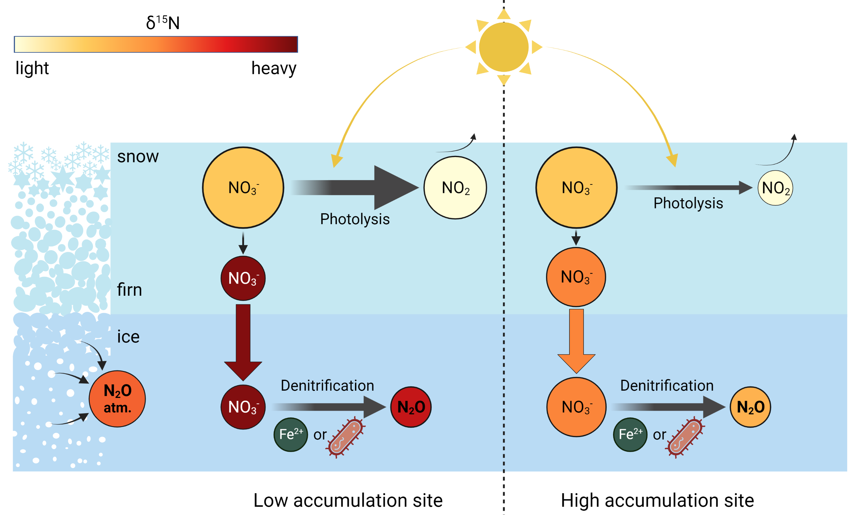
Investigating the reaction consists, first of all, in identifying the precursors and reactants. The two main production pathways for N2O are nitrification, i.e. conversion of ammonium (NH4+) to nitrate (NO3-) with N2O as a byproduct, and denitrification, i.e. reduction of NO3- to N2O (Baggs 2011). The amounts of NO3- and NH4+ in ice are both more than enough to form the observed amounts of in situ N2O. Comparing N2O data from different ice cores, we observe that in drilling sites with low snow accumulation rates the in situ fraction of N2O has high δ15N values compared to the atmospheric fraction. This is the case in the Vostok (Sowers 2001) and EDC (unpublished data) ice cores. The δ15N value of NO3-, impacted by post-depositional processes, is also higher with a decreasing accumulation rate. Indeed, NO3- photolysis in snow is accentuated in low accumulation sites, inducing high enrichment in 15N (Fig. 2; Erbland et al. 2013). These similar isotopic enrichments make NO3- a good candidate as a precursor of in situ N2O. To test this hypothesis, we are currently performing joint measurements of the nitrogen and oxygen isotopic compositions of N2O and NO3- in the same samples. The in situ fraction of N2O and its isotopic composition are calculated using a mass balance approach, with atmospheric values as defined by the almost unaffected 140-kyr record from the Talos Dome ice core (Schilt et al. 2010b). Correlated isotopic signatures of NO3- and in situ N2O would point to a denitrification reaction.
Our next step is to take a closer look at the production pathway. Denitrification can be performed by bacteria and through abiotic processes (Fig. 2). For example, NO3- is reduced to N2O by Fe2+ (Samarkin et al. 2010). As the intramolecular distribution of 15N in the N2O molecule (15N-14N-O or 14N-15N-O) only depends on the production pathway, we plan to measure the position-dependent isotope ratio of nitrogen in N2O to distinguish between a biotic or abiotic reaction.
|
|
Figure 2: Schematic of the hypothesized process of N2O in situ production in the ice. Since the snow accumulation rate controls the isotopic fractionation of NO3- photolysis, NO3- archived in ice has a different nitrogen isotopic signature at low and high accumulation sites. If NO3- is the precursor of in situ N2O, this isotopic difference is transferred to N2O through denitrification, also associated with fractionation. |
Conclusion
A precise understanding of the processes leading to N2O in situ production represents a major step forward in interpreting and completing the N2O record, which would complement the existing Antarctic CO2 and CH4 records over the last 800 kyr. Knowing the past variations of the three most important greenhouse gases is crucial to understanding the climate system, and, thus, better predict future climate change.
affiliation
1Climate and Environmental Physics, Physics Institute and Oeschger Centre for Climate Change Research, University of Bern, Switzerland
contact
Lison Soussaintjean: lison.soussaintjean@unibe.ch
references
Baggs EM (2011) Curr Opin Environ Sustain 3: 321-327
Erbland J et al. (2013) Atmospheric Chem Phys 13: 6403-6419
Fischer H et al. (2019) Biogeosciences 16: 3997-4021
Flückiger J et al. (2004) Glob Biogeochem Cycles 18: GB1020
IPCC (2021) Climate Change 2021: The Physical Science Basis. Cambridge University Press, 2391 pp
Lambert F et al. (2008) Nature 452: 616-619
Landais A, Stenni B (2021) Water stable isotopes (δD, δ18O) data from EDC ice core. PANGAEA
Prather MJ et al. (2015) J Geophys Res Atmos 120: 5693-5705
Samarkin VA et al. (2010) Nat Geosci 3: 341-344
Schilt A et al. (2010a) Quat Sci Rev 29: 182-192
Schilt A et al. (2010b) Earth Planet Sci Lett 300: 33-43
Sowers T (2001) J Geophys Res Atmos 106: 31903-31914
Spahni R et al. (2005) Science 310: 1317-1321
O2 to N2 ratios from air entrapped in ice cores are used as a proxy for insolation, providing a robust dating technique. However, many uncertainties surround the record formation due to limited understanding of the mechanisms driving the insolation signal.
Ice cores are unique archives because they contain bubbles which store samples of the atmosphere over the last several millions of years. In particular, ice cores provide records of greenhouse gas concentration (CO2, CH4, N2O). Less emphasis has been put on the reconstruction of atmospheric O2 concentration from air trapped in ice cores, despite its importance in global biogeochemical cycles. This is because the concentration of O2 in air bubbles is affected by processes associated with pore close-off (Fig. 2). We traditionally express the concentration of O2 by measuring the ratio of O2 to N2 trapped in the ice with reference to today’s atmospheric O2/N2 (denoted as δO2/N2).
In addition to providing a record of natural variability in atmospheric O2 concentrations, δO2/N2 records, both from Antarctica and Greenland, are strongly anti-correlated with local insolation intensity at the summer solstice (Fig. 1; e.g. Bender 2002). O2 in trapped gas is relatively depleted compared to N2 during periods of high insolation, and vice versa. The strong resemblance between the summer solstice insolation variability and the δO2/N2 variability paved the way for a new dating method, based on the tuning of δO2/N2 curves on the well-known curves of past local insolation. However, our understanding of the processes causing the insolation imprint are incomplete, which limits a precise reconstruction of past variability in atmospheric O2 concentration and increases uncertainty when using δO2/N2 as a dating tool.

|
|
Figure 1: δO2/N2 records covering different time periods from Dome Fuji (Kawamura et al. 2007; Oyabu et al. 2021), South Pole (Severinghaus 2019) and EPICA Dome C (Extier et al. 2018) compared to the summer solstice insolation intensity (dotted line) based on the latitude of the respective ice-core sites. All records are plotted on the respective ice-age scales. The three sites, Dome Fuji (red), South Pole (green), and Dome C (blue) are indicated on the map (Matsuoka et al. 2021). |
While this incomplete understanding does not necessarily decrease the usefulness of δO2/N2 for ice-core dating, it is important to be able to physically describe the mechanisms. In this article, we present recent and ongoing efforts to understand 1) the natural variability of O2/N2 in the atmosphere from ice-core records, and 2) the processes within the ice sheet that cause O2 to be depleted in air bubbles during high insolation periods.
Natural variability of O2/N2 in the atmosphere
At present, seasonal cycles are apparent in measurements of atmospheric O2/N2 from multiple meteorological stations. Biological productivity causes an enrichment of O2 during the summer months (photosynthesis dominated) and a decrease during winter (respiration dominated), with an inverted pattern between hemispheres due to slow inter-hemispheric mixing of air (Keeling et al. 1998). These seasonal effects are not recorded in ice-cores because of air diffusion over several years before the pore closure process. However, the seasonality is a response to productivity in the biosphere, and, thus, we may expect that long-term changes in productivity could influence absolute δO2/N2 values.
Over the past 800 kyr, a gradual decreasing trend in δO2/N2, first observed in the EPICA Dome C (EDC) record (Bazin et al. 2016; Landais et al. 2012), is apparent in various ice-core records from Antarctica and Greenland (Stopler et al. 2016). This quasi-coherence between records suggests a decrease in atmospheric O2, posited to be the result of increased rock weathering throughout the Pleistocene (Stopler et al. 2016; Yan et al. 2021). Yan et al. (2021) used discontinuous δO2/N2 measurements on 1.5-million-year-old (Myr) ice from the Alan Hills to propose that the decreasing trend in δO2/N2 may have started around the Mid-Pleistocene Transition (MPT; around 1200–800 kyr BP). They observed comparable mean δO2/N2 values between samples from 1.5 Myr and 800 kyr, thus deviating from the steady decrease in δO2/N2 of 8.4‰ per million years (Stopler et al. 2016). This poses interesting questions as to the drivers of the MPT.
Superimposed onto this long-term trend is an orbital-scale cyclicity in δO2/N2 records, which closely follows the local insolation curve for a given site. While part of this variability can be attributed to biological or geological causes, the first-order influence on this signal is believed to be rather local summer solstice insolation.
|
|
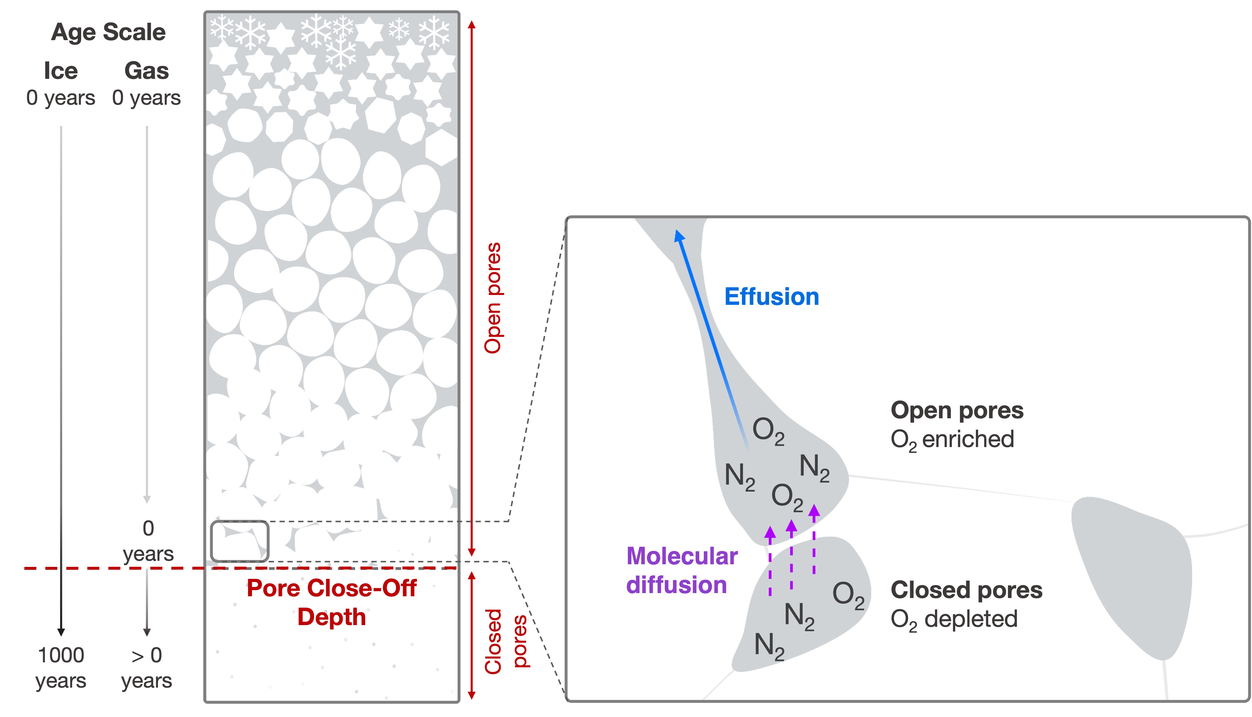
Figure 2: A diagram representing the firn column with an explanation of the two different age scales: the ice-age scale, which tells us when the ice was at the surface; and the gas-age scale, which tells us when the air was trapped in bubbles around the close-off depth. The box illustrates the two proposed mechanisms of gas loss during pore closure using a diagram modified from Severinghaus and Battle (2006). |
Insolation-driven δO2/N2 due to physical processes within the ice
Insolation-driven variations in δO2/N2 ice-core records are classically interpreted as being the result of a loss of O2 molecules from bubbles as they seal off from the atmosphere (Fig. 2; e.g. Severinghaus and Battle 2006). The formation of air bubbles occurs at about 60–120 m below the ice-sheet surface when the unconsolidated and porous snow constituting the upper part of the ice sheet has become as dense as ice. At this depth, called the close-off depth, the gases can be over 1000 years younger than the surrounding ice, resulting in separate timescales for the ice and the entrapped gases (Fig. 2). Even though δO2/N2 is measured in the air bubbles, δO2/N2 variations more strongly correlate with insolation variations when set to the ice-age scale than when set on a gas scale (Bender 2002). This observation suggests that the link between insolation and δO2/N2 in air bubbles is related to physical properties of the snow, as discussed below.
Insolation intensity modifies the properties of the snow near the ice-sheet’s surface, such that strong insolation drives snow grain growth. These near-surface modifications in snow properties persist during the snow densification process from the surface down to the close-off depth (Fig. 2), and then determine the amount of O2 lost during the pore closure process. So, by some mechanism, more O2escapes from the closing air bubble when the surrounding ice experienced strong insolation when near the surface, and vice versa. This preferential loss of O2 is called fractionation. The route by which the O2 escapes remains up for debate, but two possible processes are:
1) Effusion through thin channels
The escape of small molecules, specifically O2 in this case, through narrow channels in the ice lattice. A 3.6 Å threshold is expected given that molecules with larger diameters appear to be unaffected (e.g. N2, Kr, Xe, CO2) (Huber et al. 2006).
2) Molecular diffusion through the ice lattice
Pressure gradients between closed bubbles and neighboring open pores enable smaller molecules (O2, Ar, Ne, He) to permeate through thin ice walls, either by the breaking of hydrogen bonds, or by jumping between stable sites in the ice lattice, where the energy needed to jump depends on the size and mass of the molecule (Ikeda-Fukazawa et al. 2005; Severinghaus and Battle 2006).
Variations in insolation are expected to modify the snow grains’ physical properties that determine the channel structure and ice matrix of the deep firn, and which, in turn, modulate the O2 loss from forming bubbles (Bender 2002; Suwa and Bender 2008). However, we still lack a clear physical explanation that links the fractionation process and the physical mechanism, which results in large uncertainties being associated with the quantitative interpretation of the δO2/N2 records. Moreover, the slope of the linear regression between δO2/N2 and insolation varies between sites, suggesting that additional parameters are influencing δO2/N2 possibly relating to local climate conditions. Any mechanistic explanation would surely include climate parameters (such as accumulation rate or temperature), which have additional influences on the snow properties at the surface, and, thus, the firn properties. A 100-kyr periodicity in the δO2/N2 data from Dome C indicates a glacial-interglacial cycle imprint showing at least a long-term climatic influence (Bazin et al. 2016). Whether this is the result of physical processes or changes in atmospheric composition remains unclear.
Outlook
While many unknowns are associated with the use of δO2/N2 as a proxy for insolation, it provides an excellent ice-core dating tool, especially when considering old ice. The upcoming Beyond EPICA Oldest Ice Core project has the potential to resolve the behavior of atmospheric O2 (O2/N2) prior to the MPT by providing continuous records from the last 1.5 million years to corroborate the Alan Hills data (Yan et al. 2021).
affiliation
Laboratoire des Sciences du Climat et de l'Environnement, CNRS-CEA-UVSQ-UPS, IPSL, Gif-sur-Yvette, France
contact
Romilly Harris Stuart: romilly.harris-stuart@lsce.ipsl.fr
references
Bazin L et al. (2016) Clim Past 12: 729-748
Bender M (2002) Earth Planet Sci Lett 204: 275-289
Extier T et al. (2018) Quat Sci Rev 185: 244-257
Huber C et al. (2006) Earth Planet Sci Lett 243: 61-73
Ikeda-Fukazawa T et al. (2005) Earth Planet Sci Lett 229: 183-192
Kawamura K et al. (2007) Nature 448: 912-917
Keeling RF et al. (1998) Global Biogeochem Cycles 12(1): 141-163
Landais A et al. (2012) Clim Past 8: 191-203
Matsuoka K et al. (2021) Env Modelling and Software 140: 105015
Oyabu I et al. (2021) The Cryosphere 15: 5529-5555
Severinghaus J (2019) South Pole (SPICECORE) 15N, 18O, O2/N2 and Ar/N2. USAP Data Center
Severinghaus J, Battle M (2006) Earth Planet Sci Lett 244: 474-500
Stopler D et al. (2016) Science 353(6306): 427-1430
Age estimates using the radioactive decay of radionuclides in ice cores have the potential to verify and extend existing age scales. The method is currently limited by unexplained variations in radionuclide concentrations and the large masses of ice needed for their measurement.
Radionuclide production
Earth is constantly bombarded by a flux of cosmic rays, which consist mainly of protons and alpha particles, traveling near the speed of light. In our atmosphere, they collide with gases and set off a cascade of nuclear reactions that result in the production of a range of radionuclides, including 10Be, 14C, 26Al, 36Cl, and 81Kr. Because the atmospheric composition is dominated by nitrogen (14N) and oxygen (16O), most reactions produce radionuclides with a relative isotopic mass below 16; heavier radionuclides are much less abundant (Beer et al. 2012; Poluianov et al. 2016).
Radioactive-decay dating is best known from radiocarbon, which is however, not suitable for most ice-core dating due to its comparably short half-life of 5.73 kyr (Beer et al. 2012). Several other radionuclides have much longer half-lives (Fig. 1a), but face two major challenges. Firstly, the low abundance of most radionuclides translates into low concentrations in ice, necessitating large sample masses for their measurement, as shown in Figure 1b. Secondly, the production of all radionuclides varies over time because the cosmic-ray flux on Earth is not constant. It is subject to modulations from the varying magnetic fields of the Sun and the Earth, since protons and alpha particles are charged particles.
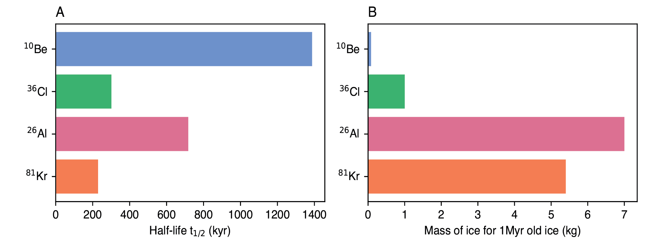 |
Figure 1: (A) Comparison of the half-lives of different radionuclides and (B) the mass of 1-Myr-old ice needed for measuring their respective concentrations. |
The advantage of radionuclide dating is that it can produce absolute age estimates, independent of other age scales and time markers. Therefore, it can also be applied to ice with a disturbed stratigraphy, making it a valuable tool for the dating of deep ice cores.
36Cl/10Be
With a half-life of t1/2 = 301 kyr, 36Cl is well suited for dating ice with ages up to 1.5 Myr, which is what the Beyond EPICA Oldest Ice Core project aims to retrieve. For a sample with an age of 1 Myr, about 1 kg of ice is needed (Fig. 1b). Variations in the production signal affect 36Cl and 10Be similarly, so taking the 36Cl/10Be ratio theoretically removes production-related variations and isolates the decay signal (Delmas et al. 2004). However, measurements from the GRIP (Yiou et al. 1997) and Dome Fuji ice cores reveal significant variations of the 36Cl/10Be ratio unrelated to radioactive decay (Fig. 2a; Kanzawa et al. 2021; ca 7450–7350 yr BP). Most likely, these variations are linked to the different chemical and physical properties of the two radionuclides, which may lead to differences in their atmospheric lifetimes, transport pathways and deposition mechanisms (Beer et al. 2012).
At low accumulation sites, 36Cl can be lost from the ice by reacting with acidic species to form volatile hydrogen chloride (HCl) after deposition, further complicating the interpretation of the measured 36Cl/10Be ratio (Delmas et al. 2004). Ice from glacial periods, however, has the potential to be unaffected by this because the glacial atmosphere contains higher concentrations of alkaline dust, which can neutralize acidic species (Röthlisberger et al. 2003; Wolff et al. 2010). Another uncertainty for age estimates is introduced by the accumulation of 10Be at grain boundaries, where it can be adsorbed on to dust particles in deep ice, creating local concentration spikes and disturbing the stratigraphic signal (Baumgartner et al. 1997; Raisbeck et al. 2006).
Nonetheless, the 36Cl/10Be ratio has been successfully used to date the deepest section of ice from the Dye3 and GRIP cores, where the age estimates agreed with other dating methods (Willerslev et al. 2007).
26Al/10Be
The advantage of using 26Al instead of 36Cl is that it quickly attaches to aerosol particles, similar to 10Be. The transport for both radionuclides should, therefore, be identical, leading to less variations in the 26Al/10Be ratio. Indeed, measurements of atmospheric air around the globe yielded the same 26Al/10Be ratio with deviations of no more than 5% and similar values for measurements in firn from several locations in Antarctica (Auer et al. 2009).
The disadvantage of using 26Al is its very low production rate, which is about 300 times lower than that of 10Be, necessitating at least 7–14 kg of ice for a single measurement of 1-Myr-old ice (Auer et al. 2009; Fig. 1b).
In a pilot study, Auer et al. (2009) measured the 26Al/10Be ratio in the deep, undated section of the EDML ice core (older than 150 kyr) and found that its values varied strongly between samples and were on average 50% higher than in samples from the modern-day atmosphere and Antarctic firn, even though the decay of 26Al (t1/2 = 717 kyr) should lead to lower values (Fig. 2b). The authors concluded that recrystallization and high pressure may result in local concentration enhancements at the bottom of the EDML core. However, these alterations and their effects on 26Al and 10Be are not understood, and the 26Al/10Be ratio, therefore, appears to suffer from a similar weakness as the 36Cl/10Be ratio: although changes in the production signal are theoretically removed, the ratio exhibits unexplained variations.
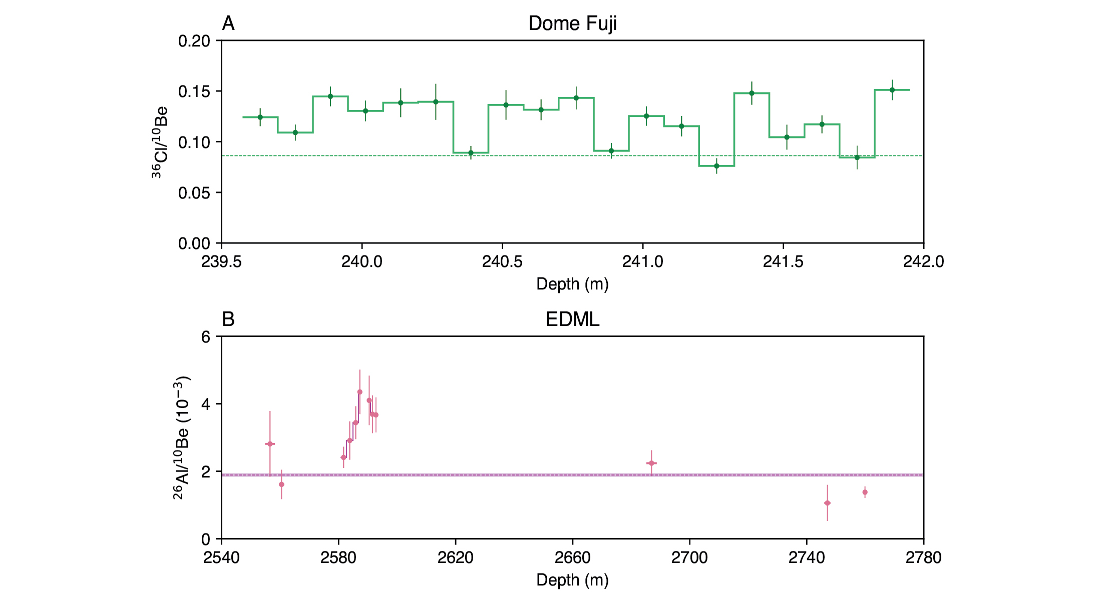 |
Figure 2: Variations of (A) the 36Cl/10Be ratio in the Dome Fuji ice core with the theoretical production rate value of 0.0862 shown as a dashed horizontal green line and (B) the 26Al/10Be ratio in the EDML ice core with the modern-day mean atmosphere value of 1.89 ± 0.05 x 10⁻³ shown as a horizontal magenta line. Data from Kanzawa et al. (2021) and Auer et al. (2009), respectively. Vertical bars indicate analytical errors. |
Using only the two deepest measurements, Auer et al. (2009) arrived at an age estimate of 670 kyr with an uncertainty of almost 40% for the deepest EDML sample, which is approximately the minimum possible uncertainty of 26Al/10Be dating with 7 kg of ice, mainly due to the low measurement efficiency.
81Kr
Contrary to the other radionuclides discussed so far, 81Kr is a noble gas, which is largely inert and remains in the atmosphere for most of its lifetime, resulting in a globally well-mixed atmospheric 81Kr/Kr ratio.
The approach for taking production variabilities into account is also different for 81Kr. Instead of using a second radionuclide to correct the signal, a reconstruction of geomagnetic field intensities is used to calculate the theoretical 81Kr/Kr ratio of the last 2 Myr (Zappala et al. 2020). This introduces uncertainties from the past cosmic-ray flux, the absorption cross sections of krypton, and the half-life of 81Kr, t1/2 = 229 ± 11 kyr. Nonetheless, the calculation of the theoretical present-day ratio agrees with measurements of modern air (Zappala et al. 2020).
First measurements of 81Kr in three deep samples of the undated Talos Dome ice-core section yielded age estimates with 9–16% uncertainty, and indicated a disturbed stratigraphy, because the deepest sample had a younger 81Kr age than the second deepest (Crotti et al. 2021).
Due to the low abundance of stable krypton (the target element for 81Kr production in the atmosphere) the production rate of 81Kr is even lower than that of 26Al. Measurements with less than 10 kg of ice became feasible only recently (Crotti et al. 2021) and current improvements aim to reduce the required sample mass to just 1 kg of 1-Myr-old ice (Ritterbusch et al. 2022).
Outlook
Several radionuclides have the potential to assist conventional dating of ice cores, especially in the deepest section, where the stratigraphy may be disturbed.
Two main issues complicate the use of radionuclide dating: uncertainty and required sample mass. For the 36Cl/10Be and 26Al/10Be ratios, variations occur over time and are not well understood, while 81Kr suffers from uncertainties connected to the calculation of the historic 81Kr/Kr ratio and its half-life. Because radioactive decay is used for dating, the required sample mass increases exponentially with age. To measure a radionuclide with consistent precision, the required sample mass doubles for each half-life.
Nonetheless, measurement techniques are constantly improving to reduce the required sample size, making radionuclide dating a more viable solution for dating old ice. Simultaneously, research aimed at a better understanding of climatic influences and post-depositional effects on the 36Cl/10Be and 26Al/10Be radionuclide ratios, as well as improved calculations of the historic 81Kr/Kr ratio, are expected to reduce the uncertainties of these three radionuclide dating methods.
affiliations
1Department of Geology, Lund University, Sweden
2Department of Earth Sciences, University of Cambridge, UK
contact
Niklas Kappelt: niklas.kappelt@geol.lu.se
references
Auer M et al. (2009) Earth Planet Sci Lett 287: 453-462
Baumgartner S et al. (1997) Nucl Instrum Methods Phys Res B 123: 296-301
Beer J et al. (2012) Cosmogenic Radionuclides. Springer, 293 pp.
Crotti I et al. (2021) Quat Sci Rev 266: 107078
Delmas R et al. (2004) Tellus Ser B 56: 492-498
Kanzawa K et al. (2021) J Geophys Res Space 126: 10
Poluianov S et al. (2016) J Geophys Res Atmos 121: 8125-8136
Raisbeck GM et al. (2006) Nature 444: 82-84
Ritterbusch F et al. (2022) 3rd IPICS Open Science Conference, Crans-Montana, Switzerland
Röthlisberger R et al. (2003) J Geophys Res Atmos 108: 1-6
Willerslev E et al. (2007) Science 317: 111-114
Wolff E et al. (2010) Quat Sci Rev 29: 285-295
Microstructure of polar ice cores provides useful information about past climate conditions, improving our understanding of Earth's history and future climate changes. The development of automated imaging systems provides efficient and high-resolution insights into ice-core microstructure and its evolution.
Deep polar ice cores drilled in Greenland and Antarctica have been used to study the Earth’s past climate, the evolution of the ice microstructure through an ice sheet, and the processes that control ice flow. As snow accumulates and turns into ice, it begins to deform and flow under the weight of the overlying snow and ice. This process, known as glacial flow, is driven by a combination of gravity and the mechanical properties of the ice itself (Binder et al. 2013; Cuffey and Paterson 2010).
Microstructure analysis of ice cores provides valuable information on the evolution of the ice sheet over time. By studying the size, shape, and orientation of individual ice crystals, we learn about the processes that control ice flow, such as deformation and recrystallization. This information helps us better understand how ice sheets respond to changes in temperature and other environmental conditions.
Over the last few decades, significant advances in computing power and digital imaging techniques have revolutionized the way we study and analyze polar ice cores. These new tools enable us to perform tasks that were once considered unfeasible or extremely time consuming, such as processing and analyzing vast amounts of data or creating continuous high-resolution images of ice-core microstructures.
From still cameras to line scanner
Recent developments in microstructure mapping have seen significant improvements: from the use of traditional still cameras and optical microscopy methods to the use of computer-controlled microscopic imaging systems. Kipfstuhl et al. (2006) provided an overview of the evolution of microstructure mapping, and how the advances in computing power and digital imaging techniques have revolutionized the way we study and analyze polar ice cores.
Early studies, such as Arnaud et al. (1998) and Nishida and Narita (1996), used still cameras to capture images of microstructures in firn and bubbly ice. Optical microscopes were also used to gather statistical data on air bubbles (Bendel et al. 2013) and air hydrates in ice (Kipfstuhl et al. 2001; Lipenkov 2000; Uchida et al. 1994). However, the use of traditional still cameras and optical microscopes had limitations in terms of image quality control and systematic mapping of microstructures.
Kipfstuhl et al. (2006) improved the process of microstructure mapping by setting up and testing a computer-controlled microscopic imaging system. The aim was to streamline and automate the microscopic observation process, resulting in scanning an ice section with dimensions of 5–10 cm x 10 cm, and generating digital images at microscopic resolution within the hour, while drilling operations were still in progress.
While the initial goal of the system was air-bubble and air-hydrate studies, Kipfstuhl et al. (2006) found that after the ice-core surface was exposed to sublimation, the method was also able to record boundaries between the ice crystals (grain boundaries) as well as a wide variety of deformation-induced features.
The microstructure analysis of ice cores dates back to 1960 when studies conducted on Camp Century and Byrd ice cores from Greenland and Antarctica, respectively, focused primarily on average grain sizes and crystal orientations (Faria et al. 2014). Later, comprehensive grain-boundary studies by Kipfstuhl et al. (2006) and Weikusat et al. (2009) led the way to the development of the first Large Area Scanning Microscope (LASM) in industry by Schäfter & Kirchoff GmbH (S+K). Subsequently, Binder et al. (2013) and Binder (2014) introduced a specialized image analysis software capable of extracting and parameterizing grain-boundary networks from LASM images.
The LASM allows for a more efficient analysis of grain boundaries. Unlike the optical microscope that requires XY translation to capture and stitch together 1500 micrographs into a map, the LASM utilizes a line scan camera, which captures images line by line, instead of a whole picture at once, and covers a larger area in a single scan (Krischke et al. 2015). Although the LASM does not need thousands of micrographs, there is still a need to stitch tens of images to cover the length of a single core (55 cm). Moreover, both systems require manual focus adjustments due to variations in the ice-sample height (Binder 2014).
The LASM, together with the Image Microstructure Analyzer software developed by Binder et al. (2014), has excellent capabilities for reconstructing the grain boundaries of the ice. This enables a detailed analysis of the spatial arrangements and characteristics of the ice grains. However, the complex sample preparation process and computationally intensive software highlight the need for further enhancements to streamline ice-core microstructure analysis.
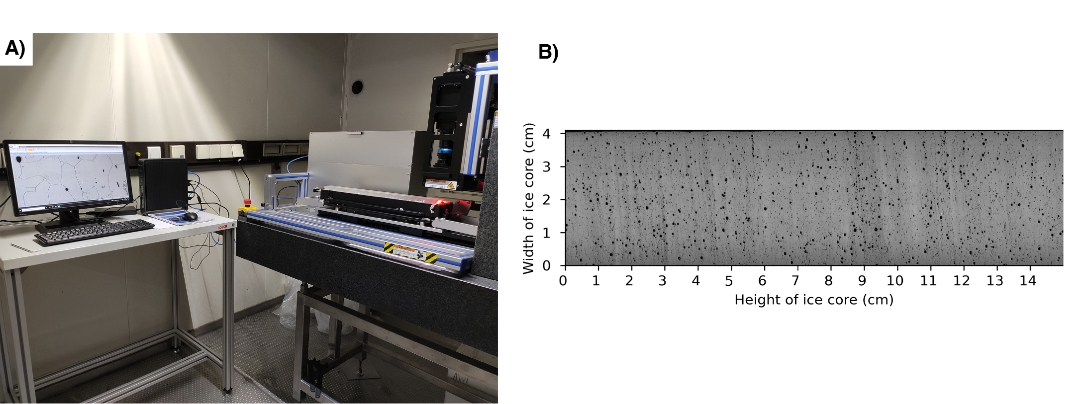
|
|
Figure 1: (A) Three-axis xLASM for the analysis of the microstructure of polar ice cores. (B) Output example of a full core scanned with xLASM from the NEEM ice core. |
Current developments in ice-core microstructure mapping
To address the issues mentioned above, ongoing testing of a second Large Area Scanning Microscope (xLASM) (Fig. 1a), which operates on three axes, aims to scan complete ice cores in a single operation. With a larger mapping area, the need for image alignment and matching is eliminated, significantly reducing computing time. Furthermore, the xLASM enables the automation of the height-focusing process.
The xLASM employs bright-field illumination. A scan of the NEEM ice core, a deep ice-core project in the Greenlandic ice cap, is shown in Figure 1b. This technique utilizes light that interacts with various components of the ice-core surface, such as grain boundaries and other microstructural features, leading to differential absorption, or scattering, of light. The transmitted light is collected by the lens and generates an image of the scanned surface. Bright regions of the sample correspond to areas that absorb or scatter light less, while darker regions correspond to areas that absorb or scatter the light more. The ice-core surface is imaged in reflection and three consecutive images of 5 μm resolution are produced in 15 minutes.
The development and optimization of the xLASM for continuous observation of crystal size structures requires a precise and smooth ice-core surface to maintain the line scanner focus. To achieve this, we have devised an experimental setup featuring an automated microtome (Fig. 2a). By sampling the entire ice core (Fig. 2b), we can streamline the labor-intensive ice-sample preparation process, minimize inconsistencies during sublimation, scan under different imaging conditions, and eliminate the image stitching procedure.
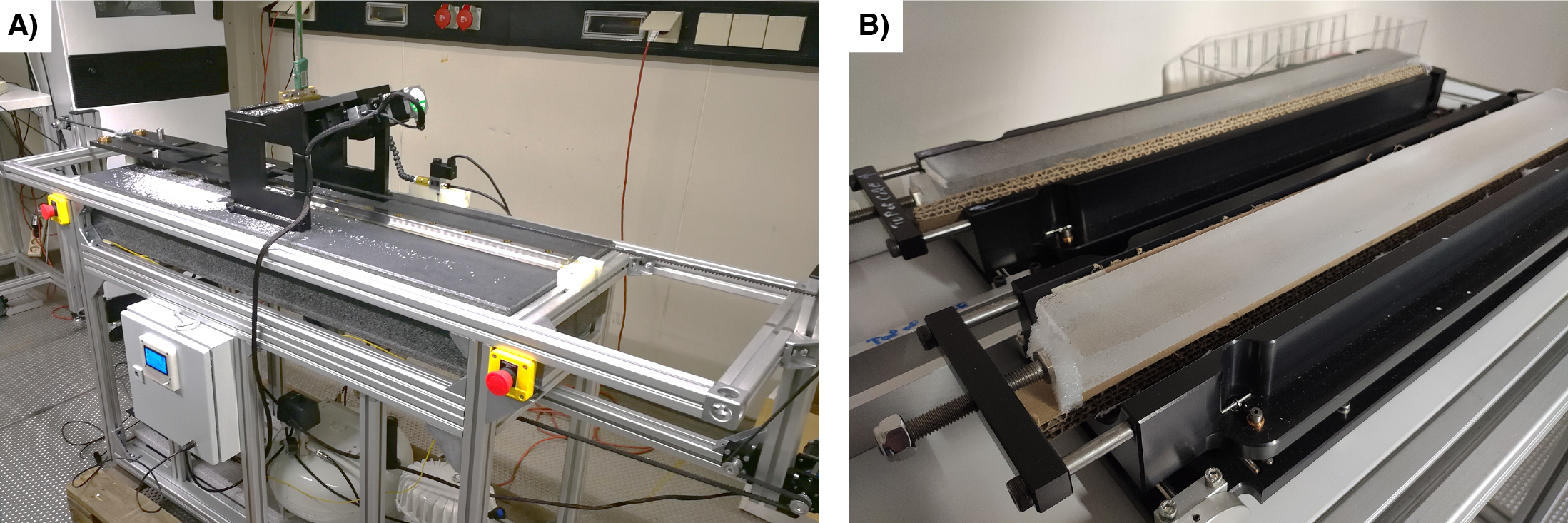
|
|
Figure 2: (A) Picture of the automated microtome, which comprises a granite plate, a linear guide for horizontal motion, and a portal housing the surgical blades. (B) Photograph of mounted ice cores left to sublimate at -20ºC after being microtomed. |
Outlook
A significant advantage of employing line scan cameras in LASMs is their ability to rapidly capture high-resolution images of ice-core microstructures with excellent contrast. Unlike the standard microscopic method, which is time consuming and computationally intensive, the innovative LASMs developed by S+K can generate high resolution ice-surface images within just 5–10 minutes. Ongoing tests involving the new xLASM, coupled with an automated microtome, enable the sampling of whole ice cores through a new processing framework.
The current setup has been tested in a cold room at -20ºC using samples from the NEEM ice core. The process of mounting, microtoming, and scanning ice cores allows for the processing of eight to 10 deep ice cores per day, aiming for more continuous ice microstructure analysis. The main time constraint is the sublimation needed to remove surface artifacts to ensure high quality data. The measurements and continuous observations obtained from the xLASM technology applied to ice cores enable the investigation of ice rheology and its impact on ice deformation. By utilizing this data, it is possible to obtain better insights on folds and disturbances in deep ice layers. This analysis is being conducted on existing ice cores and is anticipated to be applied to future ice cores obtained from the Beyond EPICA Oldest Ice Core project in Antarctica.
affiliationS
1Physics of Ice, Climate, and Earth, Niels Bohr Institute, University of Copenhagen, Denmark
2Schäfter + Kirchhoff GmbH, Germany
3Alfred Wegener Institute, Helmholtz Centre for Polar and Marine Research, Bremerhaven, Germany
4Centre for Earth Observation Science, University of Manitoba, Winnipeg, Canada
contact
Miguel Moreno: miguel.moreno@nbi.ku.dk
references
Arnaud L et al. (1998) J Glaciol 44: 326-332
Bendel V et al. (2013) J Glaciol 59: 972-980
Binder T et al. (2013) J Microsc 250: 130-141
Faria SH et al. (2014) J Struct Geol 61: 2-20
Kipfstuhl S et al. (2001) Geophys Res Lett 28: 591-594
Kipfstuhl S et al. (2006) J Glaciol 52(178): 398-406
Krischke A et al. (2015) Optik & Photonik 10: 32-35
Lipenkov VY (2000) In Hondoh T (Eds) Physics of Ice Core Records. Hokkaido University Press, 327-358
Nishida K, Narita H (1996) J Geophys Res 101: 21311-21317
The impurities contained in ice impact its physical and chemical properties. To understand this impact, and therefore improve ice-derived climate reconstructions, it is critical to determine the location and nature of impurities in the ice matrix.
The Earth’s glaciers and the Antarctic and Greenland ice sheets store a vast amount of information about its climate history. Within the ice, alongside preserved pockets of Earth’s past atmospheres and the temperature record detailed in the isotopic ratios of water molecules, impurities provide additional insights into the past. These impurities can be diverse in origin and composition, such as dust particles carried from Patagonia to Antarctica (Basile et al. 1997), ash from Icelandic volcanoes reaching Greenland (Wittmann et al. 2017), and salt aerosols originating from open waters and the surface of sea ice (Rhodes et al. 2017). These impurities are analyzed to investigate past atmospheres’ aerosol composition, the physical properties of ice, and many other subjects (Stoll et al. 2021). While analysis of meltwater has proved an excellent approach to extracting such information from ice, melting ice causes the loss of spatial data relating to the location of impurities within the ice matrix. Precise information regarding the location of these impurities within the ice matrix is crucial (Stoll et al. 2022). Understanding the location of impurities within the ice microstructure helps address questions on how to best exploit highly disturbed and thinned ice, such as that targeted at Little Dome C in Antarctica by the Beyond EPICA Oldest Ice Core project, and translate this proxy data into meaningful climate and environmental data. Both microscale processes, such as ice formation from snow, and macroscale processes, such as ice flow, are linked to how impurities are distributed in ice. These post-depositional effects impact the preservation of impurity-derived climate signals by altering the local concentrations and distribution of impurities within the ice. Ice at the bottom of the Antarctic Ice Sheet has highly thinned layers where many thousands of years of ice and impurities can be packed into a single vertical meter. This concentration of information necessitates further advancements in analytical techniques to fully exploit this archive. Work done in the DEEPICE project is developing our understanding of these topics, in part through developments of high-resolution analytical techniques to map impurities in ice. Ideally, any analysis of such ice should be micro-destructive or non-destructive to preserve the ice, enabling further analysis and retention of an archive.
Ice structure and impurity locations
A pure ice crystal is a solid arrangement of water molecules in a hexagonal structure. Glacier ice, formed by the metamorphosis of snow, comprises many such crystals. Structural discontinuities between adjacent crystals are known as grain boundaries (Fig. 1). However, glacier ice is not comprised solely of crystals containing pure water. Impurities are also incorporated in the ice and have been shown to exist both within crystals and at their boundaries (Bohleber et al. 2021). So, how are the locations of impurities in ice samples determined?
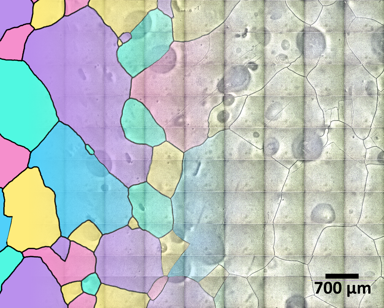
|
|
Figure 1: Optical image (right) and illustration (left) of the grain-scale structure of glacier ice collected from talos Dome, Antarctica. Glacier ice is comprised of crystals (represented in different colors in the cartoon section), which can have different orientations. the intersections of crystals (represented by black lines in the cartoon) are known as grain boundaries. Gray rounded features are air bubbles. Impurities are distributed throughout grain- interior and inter-grain regions, as illustrated in Figure 2, which shows the chemical distribution in the same area. Figure modified from bohleber et al. (2021). |
Locating impurities
To enable the analysis of samples in their solid state, and therefore understand the spatial distribution of their impurities, ice samples must be stored and analyzed at stable temperatures of -10°C or lower. Despite this challenge, several techniques have been applied to ice that shed light on the spatial distribution of impurities within the microstructure of ice. These have been discussed in detail in a review by Stoll et al. (2021). These techniques are often coupled with some optical analysis to locate targeted features such as grain boundaries or dust particles in an ice sample. Following is a discussion of three complementary techniques used to understand the spatial distribution of impurities in ice.
Raman spectroscopy uses the change in energy experienced by monochromatic incident photons interacting with a molecule’s vibrational modes to determine the chemical structure and, thus, the composition of a target. In ice analysis, Raman spectroscopy is used to determine the mineralogical composition of insoluble minerals throughout the volume of an ice sample. The output is precise information on the mineralogy of a particle at a well-defined location inside the ice, but no information is collected on soluble impurities (Stoll et al. 2022).
Scanning electron microscopy (SEM) and coupled energy dispersive X-ray spectroscopy (EDS) make use of both the secondary electrons and X-ray radiation emitted from a surface that an incident electron beam has bombarded. When used in tandem, the SEM and EDS techniques can be used to both spatially map the microstructure of ice and gain information on the composition of impurities simultaneously, but without quantifying the concentration of impurities present (Barnes et al. 2002).
Laser ablation inductively coupled plasma mass spectrometry (LA-ICP-MS) utilizes a brief laser pulse to ablate small volumes of material from a target’s surface. This material is aerosolized and transported to a mass spectrometer, where its elemental composition and relative concentration is determined. This process gives information on soluble and insoluble elements present in a target sample. By rapidly firing the laser over an area of a sample, high-resolution two-dimensional elemental maps, usually covering vertical cross-sections, can be generated. Figure 2 displays such data from an ice sample from Talos Dome, Antarctica (Bohleber et al. 2021). This image shows the impurities distribution on an ice sample’s surface at a resolution of 35 µm.
These techniques give complementary data on impurities, with the potential for retention of samples due to the non-destructive nature of Raman spectroscopy, joint SEM and EDS analysis, and the micro-destructive nature of LA-ICP-MS. By combining these approaches, a more comprehensive analysis of impurity location in ice can be achieved across different scales, encompassing both detailed particle-level information and broader spatial patterns.
Data processing
The application and improvements of the methods presented here are leading to the production of large amounts of high-quality data. Much like the data collection processes, data-analysis procedures are being adapted to process and interpret these data. Two-dimensional spatial data, such as the chemical LA-ICP-MS image shown in Figure 2, benefits greatly from analysis using automated computer image processing to perform tasks such as isolating the grain boundary network from an image, overlaying optical images over chemical images, and extracting crystal sizes (Binder et al. 2013). After extracting this information, the extensive range of spatial data embedded within these images can give valuable insights into particle compositions and impurity distribution across distinct regions of the ice matrix, allowing for a better understanding of chemical and physical processes occurring within the ice.

|
|
Figure 2: LA-ICP-MS elemental map showing the distribution of sodium on the surface of an ice sample. Note the strong association of sodium with the grain-boundary network, as seen in Figure 1, which shows an optical image of the same area. Figure generated from data presented in Bohleber et al. (2021). |
Outlook
The ice core due to be extracted from Little Dome C in Antarctica will form a continuous ice record beyond 1.5 million years ago, offering new insights into the past variability of our climate and the history of the Antarctic Ice Sheet. However, analysis of this exceptionally deep and old ice presents distinct challenges. The ice matrix and impurity record at such depths have undergone many changes during their journey down the ice sheet. The ice at the bottom of this core has thinned considerably, containing tens of thousands of years’ worth of variability within a single meter, meaning collection and interpretation of high-resolution data is crucial to fully capture the information within the core fully. Furthermore, the nature of this core as a unique archive and limited resource demands careful use. Therefore, any analysis should be high-resolution and non-destructive. Developments to the techniques discussed in this article are well-timed to give insight into the origin, composition, and location of the impurities within the core. This information will form a key part of our understanding of this exceptional climate archive.
affiliationS
1Department of Environmental Sciences, Informatics and Statistics, Ca’Foscari University of Venice, Italy
2Alfred Wegener Institute, Helmholtz Centre for Polar and Marine Research, Bremerhaven, Germany
3Department of Earth Sciences, University of Cambridge, UK
contact
Piers Larkman: piersmichael.larkman@unive.it
references
Barnes PRF et al. (2002) J Microsc 205: 118-124
Basile I et al. (1997) Earth Planet Sci Lett 146: 573-589
Binder T et al. (2013) J Microsc 250: 130-141
Bohleber P et al. (2021) The Cryosphere 15: 3523-3538
Rhodes RH et al. (2017) Atmospheric Chem Phys 17: 9417-9433
Stoll N et al. (2021) Front Earth Sci 8: 615613