High-precision sampling of laminated sediments: Strategies from Lake Suigetsu
Takeshi Nakagawa1 and Suigetsu 2006 Project Members2
High-precision depth control is an absolute necessity for varve studies. The Lake Suigetsu 2006 project developed simple yet effective solutions to the most common problems related to core preparation and archival.
Depth control is crucial for all sediment studies and very small differences, even at the mm-scale, can be critical when studying past environmental changes at high resolution. However, achieving and maintaining such precision along a long core is challenging.
Splitting a cylindrical core into sampling and archival halves is common practice, and at some point, when the sediment of the sampling half is already exploited, researchers may wish to take complementary samples from the archive half. But even the seemingly simple task of taking a sample from exactly the same position as in the sampling half is not always easy because cores can expand or contract during storage. Also, tops and bottoms of core sections do not always retain clean and flat surfaces from which precise distances can be measured.
The earlier phase of the Lake Suigetsu project (SG93) revealed such problems; however, most were resolved through innovative techniques developed during the follow-up project that started in 2006 (SG06). This article outlines how we achieved depth control with millimeter or even sub-millimeter precision on a >40 m long quasi-continuously laminated sediment core.
Sampling techniques
 |
|
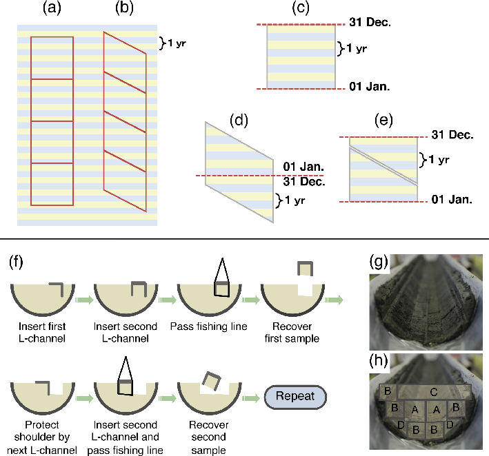
Figure 1: Top. Parallel samples (a) may contain four blue and three yellow “seasonal” layers, or vice versa, depending on sampling position, making the resulting samples incoherent. This effect is considerably reduced in diagonal samples (b). If one could cut samples precisely between 1 January and 31 December, then we would not have the “last seasonal layer” problem (c). Such ideal cutting is not possible in the real world. However, diagonal cutting is almost equivalent to such ideal cutting. Theoretically (i.e. not in practice), it is possible to cut a diagonal sample into two blocks precisely at the transition from one year to the next (d). By flipping the upper and lower blocks of (d), we can obtain a sub-sample (e), which is very close to the ideal cutting (c) in terms of the number of included seasonal layers. Bottom: (f) Procedure to recover multiple LL-channel samples (modified after Nakagawa et al. 2012) and (g-h) an example of intense sub-sampling by double-L (LL) channels. A and B: 15x15 and 12x12 mm LL-channel samples. C: Slab samples for soft X-radiography. D: 12 mm single L-channel samples. 84% of the entire core and 94% of the undisturbed part (i.e. excluding the outer 2 mm) of the core were recovered. |
It is common practice to slice varved sediments into regular thin (typically 0.5 or 1.0 cm) disks to avoid depth uncertainties between sub-samples from the same slice. However, this is not ideal because the varved sediment samples are then likely to either under- or over-represent a specific season (Fig. 1a). This is particularly a problem when producing measurements of signals with strong seasonality, i.e. most paleoclimatological proxies. If a sample represents around ten years, such as those typically used for pollen or diatom analysis, inclusion or exclusion of one seasonal layer can result in up to 10% difference in the proxy signal. Indeed, it is mainly for this reason that the pollen data from the precursor SG93 project (e.g. Nakagawa et al. 2003) had a low signal to noise ratio. A simple solution to overcome this problem of introducing a seasonal bias from arbitrarily sampling the 'last seasonal layer' is diagonal cutting. If one can avoid cutting cores into disks, but instead cut them into longitudinal bars and slice these bars diagonally into individual samples, then the “last seasonal layer” of each sample becomes blended (Fig. 1b). Or, in other words, the number of years represented in each sample becomes almost uniform for all seasons. This can be geometrically understood by flipping upper and lower parts of the same sample (Fig. 1c-e).
U-channel sampling is common, especially for paleo-magnetism studies, as a method to obtain longitudinal sediment bars from cylindrical cores. However, it is not easy to take multiple U-channel samples from the same core because the first U-channel makes an exposed fragile “shoulder”, which is very likely to be destroyed by subsequent insertion of a new U-channel. Therefore, for the SG06 project, we invented a double-L (LL) channel (Nakagawa et al. 2012). The LL-channel is almost identical to the U-channel, but consists of two L-shaped angles, which together form the “U” shape. The first L-channel protects the fragile shoulder regions. The second L-channel can then be inserted to produce the combined U-channel. Finally, the sediment underneath is cut with a fishing line to recover the sediment bar from the rest of the core. The LL-channel method allows multiple sampling of the same core section (Fig. 1f), typically allowing >90% of the undisturbed part (i.e. excluding the outer 2 mm) of the core to be recovered (Fig. 1g-h).
Another advantage of the LL-channel technique is that we can remove one of the L-channels after recovering the sample and leave the sediment sitting on only one L-channel. This exposes two sides of the longitudinal sediment bar, instead of just one, as with the U-channel. The exposure of two sides allows an easy diagonal slicing of the bar-shaped samples. This approach is much tidier than digging holes from U-channel samples and provides an almost ideal solution to the problem of the "last seasonal layer". Finally, L-shaped angles are less expensive than specifically manufactured U-channels and are easy to obtain in a range of sizes from hardware stores.
We have also developed relatively simple tools (SG06 Centi-slicer and Milli-slicer) to facilitate the diagonal slicing of LL-channel-derived samples at a regular interval of either 1 cm or 1 mm, respectively. The relevant explanatory video-clips and comprehensive description of sampling techniques can be viewed online.
Precise depth control
Because laminae are not always perfectly parallel and the samples often expand or contract depending on storage conditions, the multiple LL-channel samples do not provide perfectly identical replicates. The distance between a given pair of layers varies across multiple LL-samples from the same section. Slicing those bars at an even interval would not yield sub-samples that are stratigraphically identical. We therefore used an interpolation technique to control depth determinations at sub-millimeter precision.
 |
|
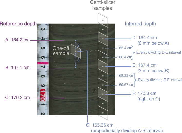
Figure 2: (A-C) Marker layers with reference depth. (D-G) Depths measured relative to the marker layer. The sediment picture is artificially distorted for demonstration purposes in order to enhance the impact of non-horizontal layers. |
The varved sediment cores from Lake Suigetsu occasionally have macroscopic layers with distinct characteristics. First, we gave numbers to these marker layers and precisely defined their depths (Fig. 2A-C) using high-resolution digital photographs taken immediately following core extraction, i.e. before any color changes through oxidation or subsequent expansion or contraction of the sediment could occur. The depth of samples bound between these marker layers is defined in one of the following ways:
• In the case of continuous sampling using the Centi-slicer, one can precisely define the depth of samples containing one of the marker layers based on the offset from that layer at the center of the sample (Fig. 2D-F). The depth of the remaining samples is then inferred by linear interpolation.
• In the case of one-off sampling (Fig. 2G), one can calculate the position of each sample by proportionally dividing the interval between two marker layers with known depths using the distances measured from the center of the sample to the nearest marker layers above and below it.
Importantly, both procedures use a defined reference depth, rather than the actual position one would measure in the laboratory. Thus, the problem of secondary expansion or contraction of cores is bypassed. The software LevelFinder has ben specifically developed for the SG06 project to facilitate all the calculations during the routine sampling described above. LevelFinder is freely available online.
SG06 Centi-slicer:
http://youtu.be/q_-D24zzzTA
http://youtu.be/LsZNVvJyaqg
SG06 Milli-slicer:
http://youtu.be/FUxLAoRGsUI
http://youtu.be/PacliEeKfSE
LL-channel sampling:
http://youtu.be/SsgYG6VNW5Q
LevelFinder:
http://dendro.naruto-u.ac.jp/~nakagawa/
affiliations
1Department of Geography, University of Newcastle, Newcastle upon Tyne, UK
2www.suigetsu.org
contact
Takeshi Nakagawa: nakag@fc.ritsumei.ac.jp
references